Chapter 2: Tokens and Embeddings
17 min readAs we’ve established, tokens and embeddings are the fundamental ways language models interact with and understand text. Without them, the magic simply doesn’t happen. Figure 2-1 in the book clearly shows this two-step process: raw text is first broken into tokens, and then these tokens are converted into numerical embeddings that capture their meaning.
Let’s begin with the first part of this process.
Section 1: LLM Tokenization
The way most of us interact with LLMs, like chatbots, we see text coming out, seemingly word by word. This output, and more importantly, the input the model receives, is processed in chunks called tokens.
- How Tokenizers Prepare the Inputs to the Language Model (Page 68-69)
- When you send a prompt to an LLM, it doesn’t see the raw string of characters directly.
- First, it passes through a tokenizer. This component breaks your input text into smaller pieces.
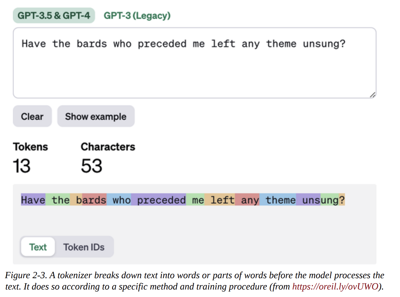
- Visual Example (Figure 2-3): The book uses the OpenAI tokenizer playground. If you input “Have the bards who preceded me left any theme unsung?”, the tokenizer might break it down into something like:
Have,the,bard,s,who,preced,ed,me,left,any,theme,unsung,?. (Note: The exact tokenization depends on the specific tokenizer used by the model.) Each of these is a token.
- Downloading and Running an LLM (Code Example Deep Dive) (Page 69-73)
- Let’s revisit the code example where we load a model (e.g., Phi-3-mini) and its tokenizer using the
transformerslibrary.# Conceptual code structure from the book # from transformers import AutoModelForCausalLM, AutoTokenizer # model = AutoModelForCausalLM.from_pretrained(...) # tokenizer = AutoTokenizer.from_pretrained(...) - When we prepare an input prompt, like:
prompt = "Write an email apologizing to Sarah for the tragic gardening mishap. Explain how it happened.<|assistant|>" input_ids = tokenizer(prompt, return_tensors="pt").input_ids - The variable
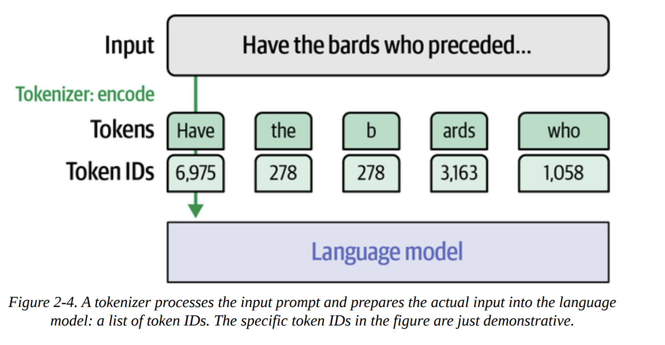
input_idsdoesn’t contain the text string. It contains a sequence of integers (a tensor), liketensor([[ 1, 14350, 385, ...]]).- Concept (Figure 2-4): Each integer is a unique ID mapping to a specific token in the tokenizer’s vocabulary. The LLM operates on these numerical IDs.
- Let’s revisit the code example where we load a model (e.g., Phi-3-mini) and its tokenizer using the
*   **Decoding Token IDs:** To see the actual tokens, we use `tokenizer.decode()` on individual IDs.
    ```python
    # for id_val in input_ids[0]:
    #     print(tokenizer.decode(id_val))
    ```
    This would print each token on a new line, showing how the original prompt was segmented.
    *   **Observations from the book's example (page 72-73):**
        *   Special tokens like `<s>` (ID 1 for Phi-3) often mark the beginning of the text.
        *   Some tokens are full words (e.g., "Write", "an", "email").
        *   Many tokens are *subwords* (e.g., "apolog", "izing", "trag", "ic"). This allows the model to handle a vast vocabulary and new words by combining known subwords.
        *   Punctuation usually gets its own token (e.g., ".").
        *   **Space Handling:** Crucially, the space character itself often isn't a distinct token. Instead, subword tokens might have a prefix (like `Ġ` in GPT-2's tokenizer, or just implied by the algorithm) indicating they are preceded by a space or are at the start of a word. Tokens without this prefix attach directly to the previous one.
*   **Output Side:** The LLM generates a sequence of *output token IDs*. The tokenizer is then used again to convert these IDs back to human-readable text. Figure 2-5 illustrates this decoding process.
How Does the Tokenizer Break Down Text? (Page 74-75) Three key factors dictate tokenization:
- Tokenization Method: Chosen by the model creators. Common methods include:
- Byte Pair Encoding (BPE): Starts with individual characters and iteratively merges the most frequent pair of bytes (or characters) to form new tokens. Used by GPT models.
- WordPiece: Similar to BPE, but merges pairs based on which new token maximizes the likelihood of the training data. Used by BERT.
- SentencePiece: Treats text as a sequence of Unicode characters and uses BPE or unigram language modeling to find optimal subword units. It’s language-agnostic.
- Unigram Language Modeling: Starts with a large vocabulary of potential subwords and iteratively removes those that contribute least to the overall likelihood of the corpus, until the desired vocabulary size is reached.
- Tokenizer Design Choices:
- Vocabulary Size: How many unique tokens will the tokenizer know? (e.g., 30k, 50k, 100k+).
- Special Tokens:
[CLS],[SEP],[PAD],[UNK],<s>,<|user|>, etc., each serving a specific purpose.
- Training Dataset: The tokenizer is trained on a large corpus of text to build its vocabulary and learn the merge rules (for BPE/WordPiece) or probabilities (for Unigram). A tokenizer trained on English will differ from one trained on Python code.
- Tokenization Method: Chosen by the model creators. Common methods include:
Word Versus Subword Versus Character Versus Byte Tokens (Page 75-78) A nice visual is Figure 2-6, showing different ways to tokenize “Have the bards who preceded…”
- Word Tokens:
- Pros: Conceptually simple.
- Cons: Large vocabulary (every word form is unique), struggles with out-of-vocabulary (OOV) words, can’t represent nuances within words (e.g., “apology” vs “apologize”). Less common now for LLMs.
- Subword Tokens: (Most common for modern LLMs)
- Pros: Balances vocabulary size and expressiveness. Can represent OOV words by breaking them into known subwords. More efficient for model context length.
- Cons: Can sometimes break words in unintuitive ways.
- Character Tokens:
- Pros: Smallest possible vocabulary, no OOV words.
- Cons: Sequences become very long, making it harder for the model to learn long-range dependencies. Less information per token.
- Byte Tokens:
- Pros: Truly “tokenization-free” in a sense, handles all Unicode characters naturally. Good for highly multilingual or noisy data. GPT-2’s BPE uses byte-level operations as a fallback.
- Cons: Sequences can also be long, less semantically meaningful units initially.
- Word Tokens:
Comparing Trained LLM Tokenizers (Page 78-91) This is a fantastic section in the book that builds intuition. The key takeaway is that different models use different tokenizers, and these choices profoundly impact how the model “sees” and processes text.
- The book takes a sample string with capitalization, emojis, non-English text, code-like syntax, and numbers.
- BERT (uncased): Loses capitalization, newlines. Emojis/Chinese become
[UNK]. - BERT (cased): Preserves case, but “CAPITALIZATION” might become 8 tokens.
- GPT-2: Handles newlines, capitalization. Emojis/Chinese are represented by multiple byte-level fallback tokens (often shown as
�but reconstructible). Handles whitespace more granularly. - Flan-T5 (SentencePiece): Loses newlines/whitespace tokens, emojis/Chinese become
<unk>. - GPT-4: Very efficient. Fewer tokens for many words. Has specific tokens for longer sequences of whitespace. Understands Python keywords like
elifas single tokens. - StarCoder2 (code-focused): Special tokens for code context (
<filename>). Each digit is a separate token (e.g., “600” -> “6”, “0”, “0”). - Galactica (science-focused): Special tokens for citations (
[START_REF]), reasoning (<work>). Handles tabs as single tokens. - Phi-3/Llama 2: Use special chat tokens like
<|user|>,<|assistant|>. - The side-by-side comparison table on pages 90-91 is incredibly illustrative.
Tokenizer Properties (Recap of factors affecting tokenization) (Page 91-93)
- Tokenization methods (BPE, WordPiece, etc.).
- Tokenizer parameters (vocab size, special tokens, handling of capitalization).
- The domain of the data (English text vs. code vs. multilingual).
- Example: A text-focused tokenizer might tokenize code indentation inefficiently (e.g., four spaces as four separate tokens), while a code-focused tokenizer might have a single token for “four spaces.” This makes the model’s job easier for code generation.
Section 2: Token Embeddings
Now that we have tokenized our text into a sequence of token IDs, the next step is to convert these IDs into meaningful numerical representations – embeddings.
- A Language Model Holds Embeddings for the Vocabulary of Its Tokenizer (Page 95)
- When an LLM is pretrained, it learns an embedding vector for each token in its tokenizer’s vocabulary.
- This collection of vectors forms an embedding matrix (or embedding layer) within the model (as shown in Figure 2-7).
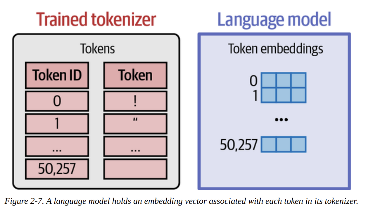
* Initially, these vectors are random, but during pretraining, their values are adjusted so that tokens with similar meanings or that appear in similar contexts have similar embedding vectors. These are *static* embeddings – each token ID always maps to the same initial vector.
- Creating Contextualized Word Embeddings with Language Models (Page 96-99)
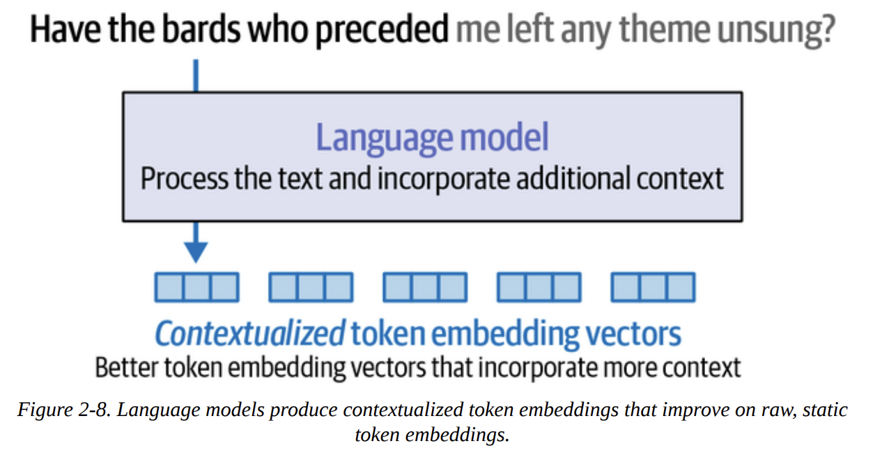
- Static token embeddings are just the starting point. The real power comes when the language model processes these static embeddings in the context of the entire input sequence.
- The output of the main Transformer blocks (before the final prediction layer) for each input token is its contextualized word embedding. This means the embedding for “bank” in “river bank” will be different from “bank” in “money bank.”
- Visual (Figure 2-8 & 2-9): Raw, static token embeddings go into the language model. The model’s layers process these, considering the whole sequence (via attention, which we’ll detail in Chapter 3). The output for each token position is a new, richer, contextualized embedding vector.
*   *Code Example (using DeBERTa, page 97):*
    ```python
    # from transformers import AutoModel, AutoTokenizer
    # tokenizer_deberta = AutoTokenizer.from_pretrained("microsoft/deberta-base")
    # model_deberta = AutoModel.from_pretrained("microsoft/deberta-v3-xsmall")
    # tokens_deberta = tokenizer_deberta('Hello world', return_tensors='pt')
    # output_embeddings = model_deberta(**tokens_deberta)[0]
    # print(output_embeddings.shape) # e.g., torch.Size([1, 4, 384])
    ```
    This `output_embeddings` tensor contains the contextualized embeddings for each token (including special ones like `[CLS]` and `[SEP]`). These are the representations used for downstream tasks or further generation.
Section 3: Text Embeddings (for Sentences and Whole Documents)
While token embeddings are crucial for the internal workings of LLMs, many applications need a single vector representation for an entire sentence, paragraph, or document.
- Concept (Figure 2-10): An embedding model takes a piece of text and outputs a single vector that captures its overall meaning.
- Methods:
- A simple approach is to average the contextualized token embeddings of all tokens in the text.
- However, high-quality text embedding models (often called Sentence Transformers or bi-encoders, building on architectures like SBERT) are specifically trained for this task. They often outperform simple averaging.
- Using
sentence-transformerslibrary (page 101-102):This gives a single vector for the entire sentence. These sentence/document embeddings are powerful for:# from sentence_transformers import SentenceTransformer # sbert_model = SentenceTransformer("sentence-transformers/all-mpnet-base-v2") # sentence_vector = sbert_model.encode("This is the best movie ever!") # print(sentence_vector.shape) # e.g., (768,)- Semantic search (as we’ll see in Chapter 8)
- Clustering (Chapter 5)
- Classification (Chapter 4)
- Text similarity tasks.
Section 4: Word Embeddings Beyond LLMs
This section briefly revisits older but foundational embedding techniques, primarily to set the stage for understanding contrastive learning, a key concept for training modern embedding models (which we’ll hit hard in Chapter 10).
Using pretrained Word Embeddings (word2vec, GloVe) (Page 103)
- Libraries like
gensimallow you to download and use classic pretrained word embeddings. - Example: Loading
glove-wiki-gigaword-50and finding similar words to “king”.# import gensim.downloader as api # glove_model_gensim = api.load("glove-wiki-gigaword-50") # print(glove_model_gensim.most_similar("king"))
- Libraries like
The Word2vec Algorithm and Contrastive Training (Page 103-107)
- Recap: Word2vec learns embeddings by predicting context words (Skip-gram) or a target word from its context (CBOW).
- Key Idea: Contrastive Approach.
- Positive Pairs: Words that actually appear near each other in the training text (e.g., “Thou” and “shalt” in the Dune example, Figure 2-11).
- Negative Pairs: Words that don’t usually appear together. These are generated by taking a context word and pairing it with a randomly sampled word from the vocabulary (Figure 2-13).
- Training Objective: The model (a simple neural network) is trained to output a high score for positive pairs and a low score for negative pairs. During this process, the embedding vectors for each word (which start random, Figure 2-15) are adjusted (Figure 2-16).
- Relevance: This “learning by contrast” is fundamental. It teaches the model not just what words are similar, but also what makes them distinct.
Embeddings for Recommendation Systems (Page 108-113)
- A practical example of applying word2vec-like thinking beyond text.
- Idea: Treat songs as “words” and playlists as “sentences.”
- If two songs frequently appear in the same playlists, their learned “song embeddings” will be similar.
- Dataset: The book uses playlists from US radio stations (Figure 2-17).
- Process:
- Prepare data: List of playlists, where each playlist is a list of song IDs.
- Train a
Word2Vecmodel fromgensimon these playlists. - Use
model.wv.most_similar()to find songs similar to a given song ID.
- The example (pages 109-113) shows this working well for recommending similar artists/genres.
Chapter 2 Summary
To quickly summarize the key takeaways from Chapter 2:
- Tokenizers are the first crucial step, breaking raw text into token IDs. The choice of tokenizer and its parameters significantly affects how an LLM processes information. Subword tokenization is the most common.
- Token Embeddings are the initial (often static) numerical representations of these tokens, learned during pretraining.
- Language models then create Contextualized Word Embeddings, which are dynamic and reflect the meaning of a token within its specific sentence.
- Text Embeddings provide a single vector for an entire sentence or document, crucial for many downstream tasks and often produced by specialized models like Sentence Transformers.
- The principles of Contrastive Learning (as seen in word2vec and later in SBERT) are fundamental for training effective embedding models by teaching them similarity and dissimilarity.
- These embedding concepts are versatile and can be applied beyond text, for example, in recommendation systems.
Ah, an absolutely brilliant question! This gets to the very heart of building practical, effective search systems. It’s a classic “new vs. old” and “meaning vs. keywords” debate, but as with most things in science and engineering, the real answer is nuanced.
Let’s break this down using my favorite approach: understanding what each one is ultimately trying to achieve.
Imagine you have two librarians.
Librarian A (The Sparse Embeddings Librarian): This librarian is a master of the old-school card catalog. They haven’t read every book, but they have meticulously indexed every single one. If you ask them for books containing the exact phrase “thermonuclear astrophysics,” they will instantly pull every card for every book that has that precise phrase. They are incredibly fast and precise for keyword matching. They are literal.
Librarian B (The Dense Embeddings Librarian): This librarian has read every single book in the library. They have a deep, intuitive understanding of the concepts and themes. If you ask them, “I want to read about how stars create energy,” they might not find any books with that exact phrase. Instead, they’ll hand you books on “stellar nucleosynthesis,” “nuclear fusion in stellar cores,” and yes, “thermonuclear astrophysics.” They understand the semantic meaning behind your query.
This analogy captures the fundamental difference. Let’s formalize it.
What They Are & How They Work
Sparse Embeddings (e.g., TF-IDF, BM25)
- What they are: These are typically very long vectors, with a dimension for every unique word in your entire vocabulary (could be 50,000+ dimensions). The key is that for any given document, most of the values in this vector are zero. The only non-zero values correspond to the words actually present in that document.
- How they work: The values are not learned in a deep neural network. They are calculated based on word frequencies. A common method is TF-IDF (Term Frequency-Inverse Document Frequency).
- Term Frequency (TF): How often does a word appear in this document? (More often = more important).
- Inverse Document Frequency (IDF): How rare is this word across all documents? (Rarer = more important and specific).
- The final score is a multiplication of these. Common words like “the” and “a” get a low score, while specific keywords get a high score.
- What they ultimately achieve: They create a representation that excels at lexical matching. They tell you which documents contain the exact words you’re looking for, and give more weight to the rare, important keywords.
Dense Embeddings (e.g., from BERT, Sentence-Transformers)
- What they are: These are much shorter vectors (e.g., 384, 768, or 4096 dimensions). The key is that nearly all values are non-zero. Each value represents some abstract, learned feature of the text.
- How they work: As we saw in Chapter 2, these vectors are the output of a deep neural network (like a Transformer) that has been trained on vast amounts of text. The training process forces the model to learn the relationships between words, concepts, and contexts.
- What they ultimately achieve: They create a representation that excels at semantic matching. They capture the meaning and intent behind the text, allowing you to find documents that are conceptually similar, even if they don’t share any keywords.
when should we use dense embeddings and when should we use sparse embeddings?
When to Use Which? The Practical Guide
This is the core of your question. Here’s a breakdown of the scenarios:
Use DENSE Embeddings when:
You need to search by concept or meaning. This is the killer use case. The user doesn’t know the exact keywords. They’re exploring a topic.
- Query: “ways to make coffee at home without a machine”
- Dense search finds: “Guide to pour-over brewing,” “How to use an AeroPress,” “The perfect French Press.” (Notice the lack of keyword overlap).
You need to handle synonyms and varied language. Your query needs to match documents regardless of the specific phrasing.
- Query: “car problems”
- Dense search finds: “automobile issues,” “engine trouble,” “vehicle maintenance.”
You are building recommendation or clustering systems. You want to group items (articles, products, songs) by their “vibe” or conceptual similarity, not just their keyword descriptions. This is what we did with the song recommender in Chapter 2.
You are dealing with multilingual content. A well-trained multilingual dense model can map queries in one language to documents in another if they are semantically equivalent.
Use SPARSE Embeddings when:
You need exact keyword matching and precision. This is where sparse models often outperform dense ones. The user knows exactly what they are looking for.
- Query:
"Interstellar" Kip Thorne - Sparse search finds: Documents that explicitly contain both “Interstellar” and “Kip Thorne.” A dense model might get confused and bring up documents about other sci-fi movies or other physicists.
- Other examples: Searching for a specific error code
E-1022, a product SKUX5A-7B2, or a legal term"res judicata".
- Query:
Your domain has a lot of specific jargon or codes. Sparse models treat every word as distinct, which is perfect for domains where
product_v1andproduct_v2are completely different things, even though a dense model might see them as semantically very similar.Interpretability is important. With sparse models, you can easily tell why a document was retrieved: it contained the specific keywords from the query. With dense models, the “similarity” is an abstract mathematical concept, making it a black box.
You need a computationally cheap and fast baseline. Sparse methods like BM25 are very fast and don’t require GPUs or large models. They are an excellent first step in any search system.
The Best of Both Worlds: Hybrid Search
So, which one do we choose? In the real world, you don’t have to. The most robust and state-of-the-art search systems – the ones powering RAG in major companies – use a hybrid approach.
This is the two-stage process we hinted at in Chapter 8:
Stage 1: Retrieval (Recall-focused): Cast a wide net to get all potentially relevant documents. You do this by running both a sparse search (like BM25) and a dense search in parallel. You then take the results from both and combine them into a larger candidate set. This ensures you get both the documents that match keywords exactly and the ones that are conceptually similar.
Stage 2: Reranking (Precision-focused): Now that you have a smaller candidate set (say, the top 100 documents from Stage 1), you use a more powerful and computationally expensive model – like a cross-encoder reranker – to precisely score the relevance of each candidate to the original query and give you the final, beautifully ordered list.
Here is a summary table for a quick reference:
| Characteristic | Sparse Embeddings (e.g., TF-IDF, BM25) | Dense Embeddings (e.g., SBERT) |
|---|---|---|
| What It Is | A very long vector, mostly zeros. | A shorter vector, all values are meaningful. |
| How It Works | Counts word frequencies & rarity (lexical). | Learned from a deep neural network (semantic). |
| Core Strength | Keyword Matching & Precision. | Meaning & Context Understanding. |
| Key Weakness | Fails if keywords don’t match (no synonym handling). | Can miss exact keyword matches; can be a black box. |
| Use When… | You need exact matches (product codes, legal terms, names). | You need to understand user intent & concepts. |
| The Winner? | Neither. The best systems use a hybrid approach, combining both for retrieval, often followed by a reranker. |
So, when you think about the “Retrieval” in RAG, don’t think of it as just one method. It’s a sophisticated pipeline that almost always benefits from using the speed and precision of sparse embeddings alongside the deep semantic understanding of dense embeddings.