Chapter 3: Looking Inside Large Language Models
15 min readNow, we address the main event: what happens after tokenization? How does a model like the Transformer take those initial embeddings and generate coherent, often brilliant, text? That’s our mission for today.
As the book mentions, we’ll start by loading our model, just to have it ready. This is the same microsoft/Phi-3-mini-4k-instruct model we’ve seen before. It’s a powerful yet manageable model that’s perfect for our hands-on exploration.
import torch
from transformers import AutoModelForCausalLM, AutoTokenizer, pipeline

# Load model and tokenizer
tokenizer = AutoTokenizer.from_pretrained("microsoft/Phi-3-mini-4k-instruct")

model = AutoModelForCausalLM.from_pretrained(
    "microsoft/Phi-3-mini-4k-instruct",
    device_map="cuda",
    torch_dtype="auto",
    trust_remote_code=True,
)

# Create a pipeline
generator = pipeline(
    "text-generation",
    model=model,
    tokenizer=tokenizer,
    return_full_text=False,
    max_new_tokens=50,
    do_sample=False,
)
With our tools at the ready, let’s start with a high-level view and peel back the layers one by one.
An Overview of Transformer Models
The Inputs and Outputs of a Trained Transformer LLM
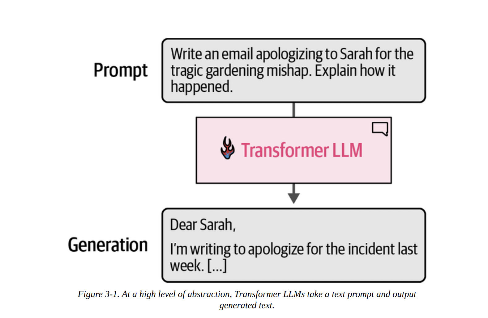
At the highest level of abstraction, a generative LLM is a system that takes a text prompt as input and produces a text generation as output. Think of it as a highly sophisticated text completion machine. Figure 3-1 shows this perfectly: you provide a prompt, and the Transformer LLM generates a relevant completion.
However, a crucial point often missed is that this generation is not instantaneous. The model doesn’t produce the entire email in one go. As Figure 3-2 shows below, the process is sequential.
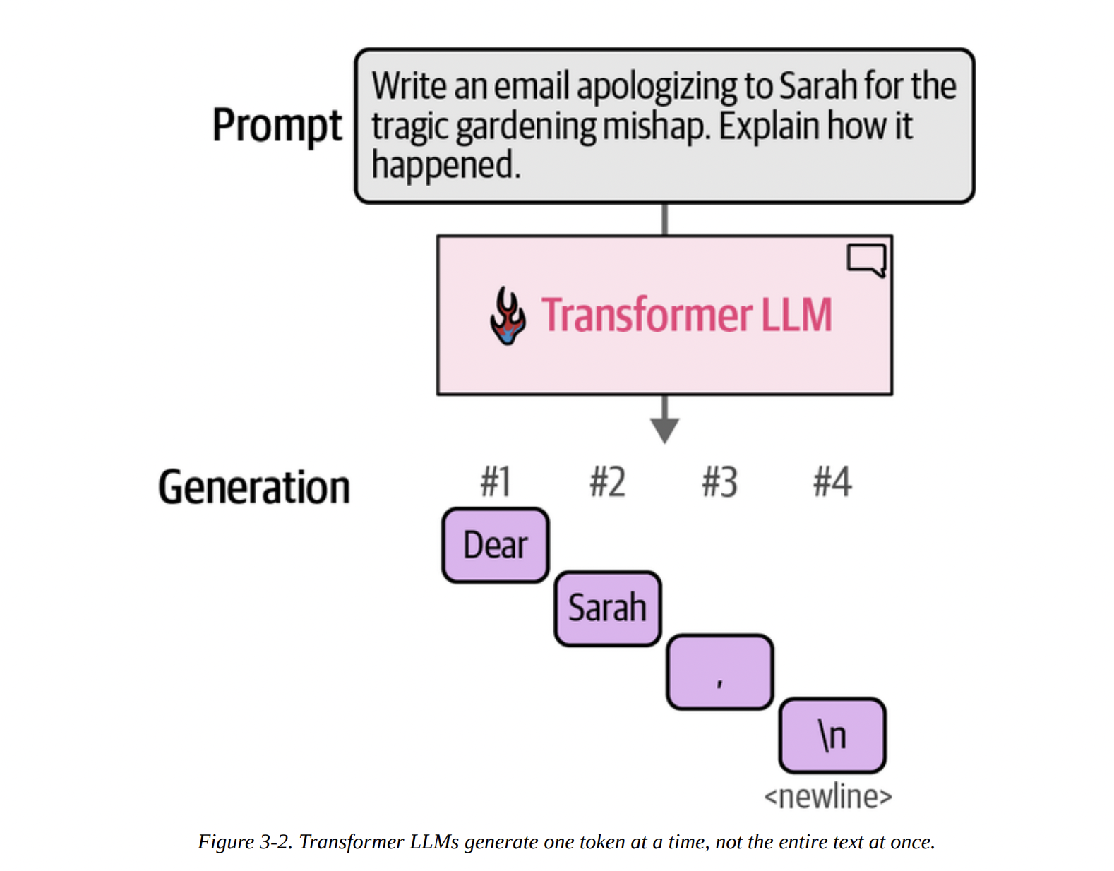
\n), and so on.
This brings us to one of the most important concepts for generative models.
Autoregressive Generation
Look at Figure 3-3 below. It shows that after the model generates the first token (“Dear”), that token is appended to the original prompt.
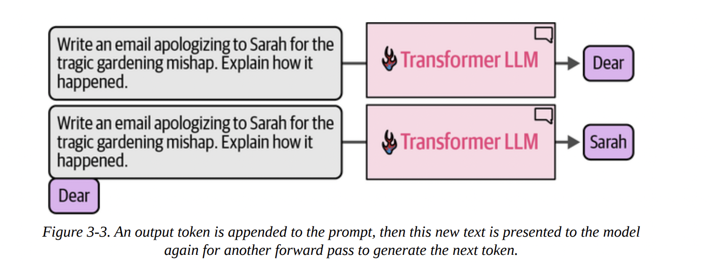
This process, where a model’s own previous outputs are fed back in as inputs for subsequent steps, is called autoregression. This is the core mechanism of generative LLMs. They are, fundamentally, autoregressive models. This is what we’re seeing when we run the generator pipeline from the book:
prompt = "Write an email apologizing to Sarah for the tragic gardening mishap. Explain how it happened."
output = generator(prompt)
print(output[0]['generated_text'])
The output begins, token by token, until it hits the max_new_tokens limit we set.
Subject: My Sincere Apologies for the Gardening Mishap...
The software wrapper around the neural network (in this case, the pipeline) handles this loop for us, but it’s essential to know it’s happening.
The Components of the Forward Pass
So, what’s inside this “Transformer LLM” box that allows for this token-by-token generation? As we can see in Figure 3-4 below, there are three main components working in concert during a single “forward pass” (the process of taking an input and producing an output):
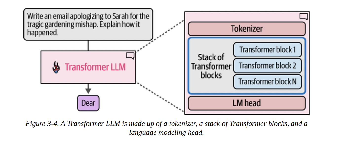
- Tokenizer: We know this from Chapter 2. It converts the input text into a sequence of token IDs.
- Stack of Transformer Blocks: This is the computational core of the model. It’s a deep stack of identical layers that process the token embeddings. This is where the “magic” of understanding context happens.
- Language Modeling (LM) Head: This is the final layer. It takes the processed information from the Transformer blocks and converts it into a usable output: a probability score for every single token in the vocabulary.
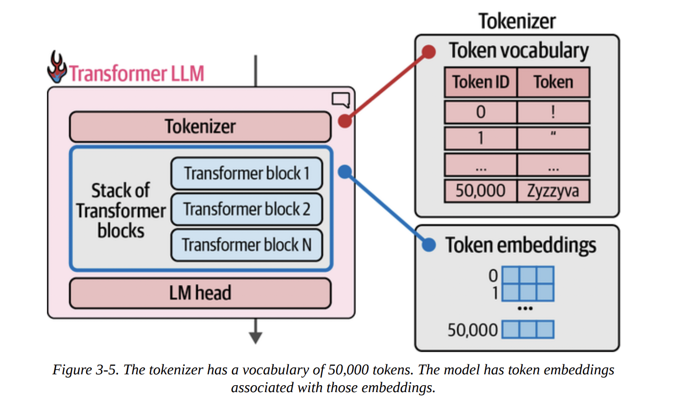
Figure 3-5 beautifully illustrates the connection we established in Chapter 2. The tokenizer has a vocabulary (a lookup table of token IDs to token strings), and the model has a corresponding token embeddings matrix. For every token ID from the tokenizer, we fetch its embedding vector to feed into the model.
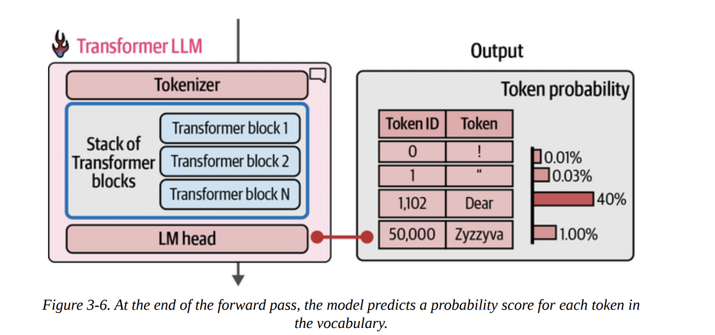
The computation flows from top to bottom. The input token IDs are converted to embeddings, which then pass through the entire stack of Transformer blocks. Finally, as shown in Figure 3-6 below, the LM head takes the final processed vector and outputs a probability distribution over the entire vocabulary. In this example, “Dear” has a 40% probability of being the next token, “Title” has 13%, and so on.
Let’s look at the model structure itself, as the book does on page 8. When we print the model variable, we see the architecture laid out for us.
Phi3ForCausalLM(
  (model): Phi3Model(
    (embed_tokens): Embedding(32064, 3072, padding_idx=32000)
    (layers): ModuleList(
      (0-31): 32 x Phi3DecoderLayer(...)
    )
    ...
  )
  (lm_head): Linear(in_features=3072, out_features=32064, bias=False)
)
Let’s break this down like a senior scientist:
(embed_tokens): This is our embedding matrix. It has 32,064 rows, one for each token in the vocabulary. Each token is represented by a vector of 3,072 dimensions. This is thed_modelor model dimension.(layers): This is our stack of Transformer blocks. We see it’s aModuleListcontaining 32 identicalPhi3DecoderLayerblocks.(lm_head): This is our language modeling head. It’s a simpleLinearlayer. Notice its dimensions: it takes an input vector of sizein_features=3072(the output from the last Transformer block) and projects it to an output vector of sizeout_features=32064(one score for each token in the vocabulary). This output vector is what we call the logits.
Choosing a Single Token from the Probability Distribution (Sampling/Decoding)
The LM head gives us logits, which can be converted to probabilities (usually via a softmax function). Now, how do we pick just one token from this distribution? This is the decoding strategy.
- Greedy Decoding: The simplest method, as shown in Figure 3-7 below, is to always pick the token with the highest probability. This is fast and deterministic, but often leads to repetitive and boring text. This is what happens when we set
do_sample=Falseortemperature=0.
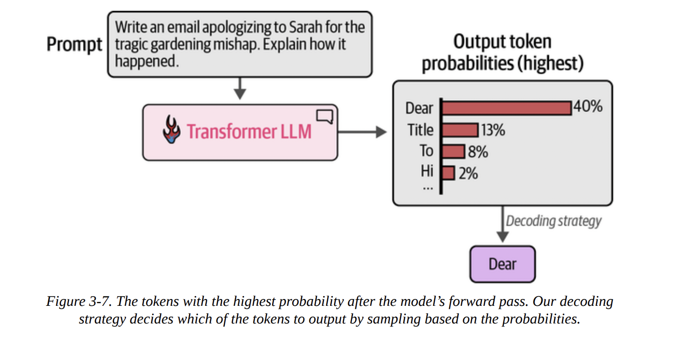
- Sampling: A better approach is to sample from the distribution. A token with a 40% probability gets picked 40% of the time. This introduces randomness and creativity. We’ll explore this more in Chapter 6.
Let’s trace this with the book’s code example. We can get the raw output (logits) from the LM head.
prompt = "The capital of France is"
# Tokenize the input prompt
input_ids = tokenizer(prompt, return_tensors="pt").input_ids.to("cuda")

# Get the output of the model before the lm_head
# Note: model.model gets the raw Transformer block outputs
model_output = model.model(input_ids)

# Get the output of the lm_head (the logits)
lm_head_output = model.lm_head(model_output[0])
The lm_head_output tensor has a shape of [1, 6, 32064]. This means:
1: A batch size of 1 (one prompt).6: Sequence length of 6 tokens (“The”, “capital”, “of”, “France”, “is”, and a special start token).32064: The logit score for each token in the vocabulary.
We only care about predicting the next token, so we look at the logits for the last input token (is). We can get this with lm_head_output[0, -1]. Then, we find the index (token ID) with the highest score using .argmax().
# Get the token ID with the highest score from the last position's logits
token_id = lm_head_output[0, -1].argmax(-1)
# Decode the ID back to text
tokenizer.decode(token_id)
And the output is, unsurprisingly, Paris.
Parallel Token Processing and Context Size
A key reason Transformers superseded older architectures like RNNs is their ability to process tokens in parallel. As Figure 3-8 intuits below, when you input a prompt, the model creates a separate processing “stream” or “track” for each token simultaneously.
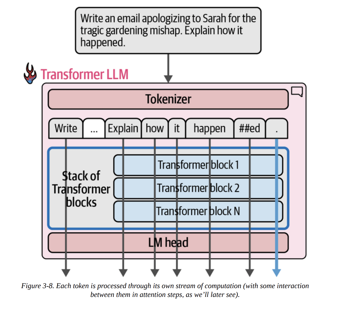
There’s a limit to how many tokens can be processed at once, known as the context length or context window. Our Phi-3-mini-4k-instruct model has a 4K (4096) context length.
As Figure 3-9 shows below, each of these parallel streams takes an embedding vector as input and, after passing through all the Transformer blocks, produces a final output vector. Crucially, for text generation, we only use the output vector of the very last token to feed into the LM head.
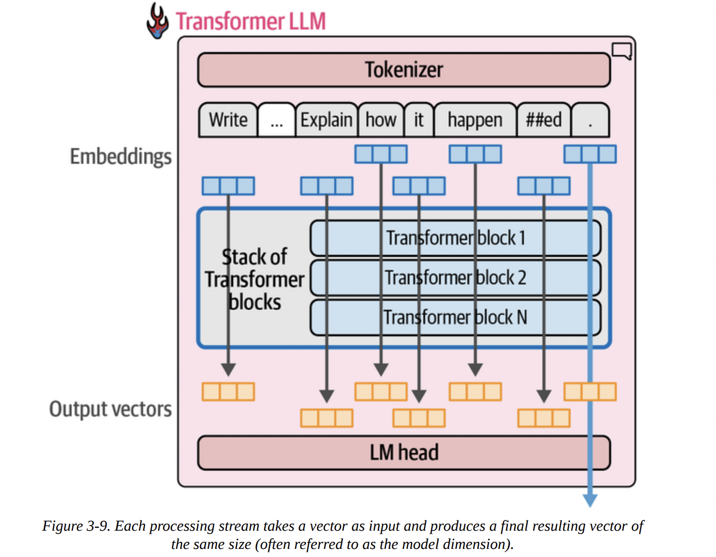
“Wait,” you might ask, “if we only use the last output, why do we bother computing all the previous ones?” That’s an excellent question. The answer lies in the attention mechanism. The computation of the final stream depends on the intermediate calculations from all the previous streams. They talk to each other inside each Transformer block.
Speeding Up Generation by Caching Keys and Values
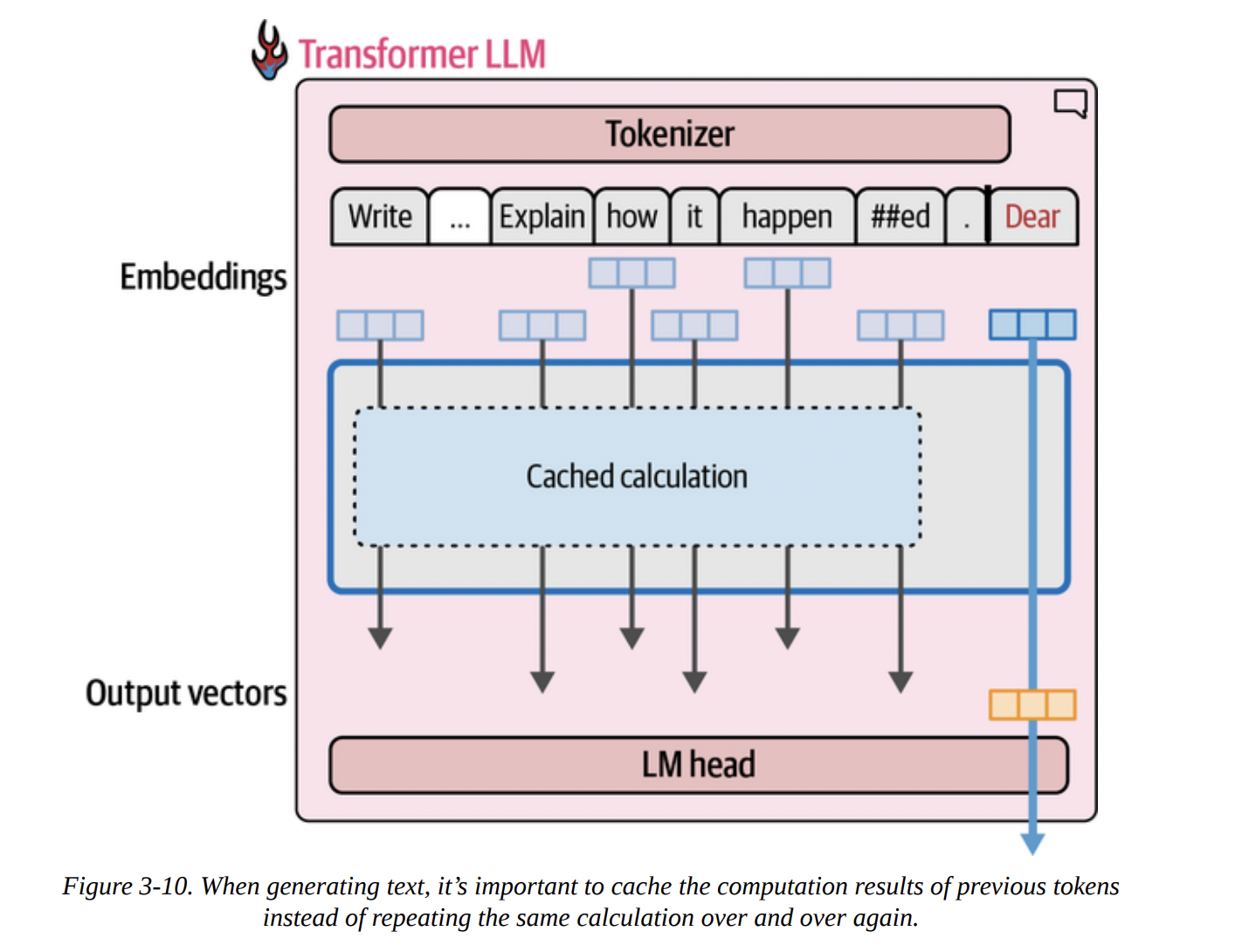
Remember our autoregressive loop? Generate a token, append it, re-process everything. This is incredibly inefficient! When generating the 100th token, we would re-calculate the streams for the first 99 tokens from scratch.
This is where the Key-Value (KV) Cache comes in. It’s a critical optimization. Inside the attention mechanism (which we’ll dissect next), certain intermediate results called “Keys” and “Values” are calculated for each token. Instead of re-calculating them every time, we can cache them.
As Figure 3-10 visualizes below, when generating the second token, we don’t re-run the calculation for the first. We retrieve its cached Keys and Values and only perform the full computation for the new token.
The book’s %%timeit example is a fantastic demonstration of this. Generating 100 tokens:
- With KV Cache (
use_cache=True): 4.5 seconds - Without KV Cache (
use_cache=False): 21.8 seconds
A dramatic, nearly 5x speedup! This is why KV caching is enabled by default and is essential for making LLM inference practical.
Inside the Transformer Block
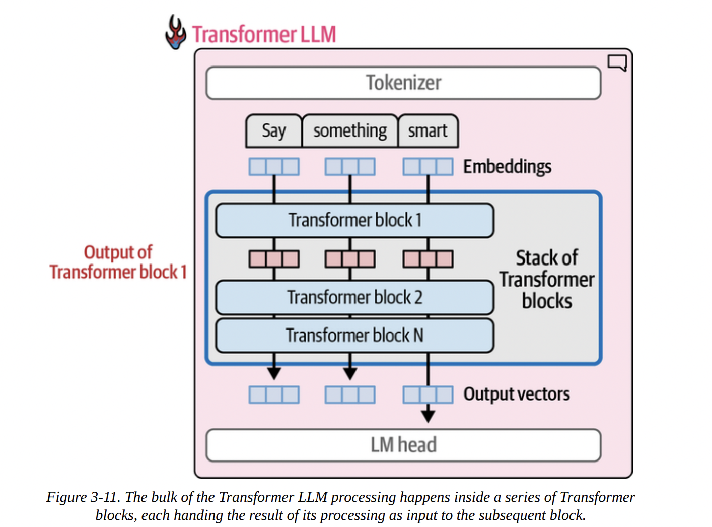
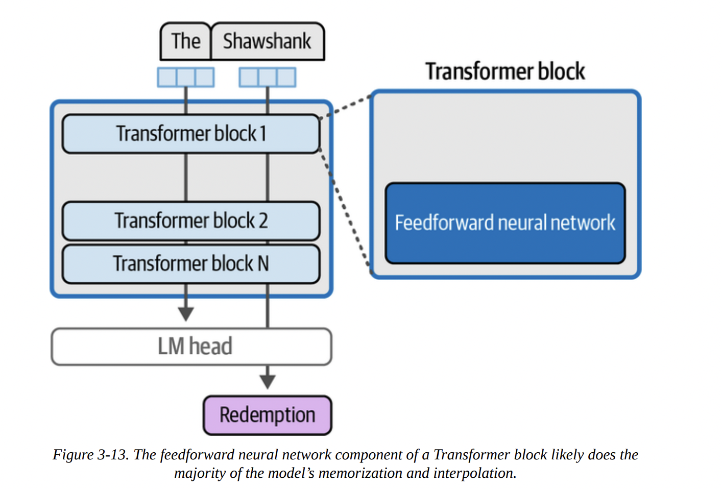
Now, let’s zoom in further. Figure 3-11 shows the processing flow: an embedding goes into Block 1, the output of Block 1 goes into Block 2, and so on.
According to Figure 3-12 below, each Transformer block is composed of two main sub-layers:
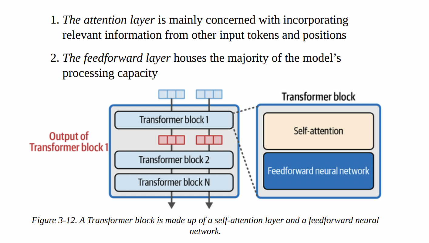
- The Attention Layer: Its job is to incorporate context. It allows a token to “look at” other tokens in the sequence and pull in relevant information.
- The Feedforward Layer (FFN): This is a standard neural network that acts as the model’s “thinking” or processing workhorse. This is where a lot of the learned knowledge is stored and applied.
The “Shawshank Redemption” example in Figure 3-13 gives a good intuition for the FFN’s role. The knowledge that “Redemption” follows “The Shawshank” is likely stored within the weights of these FFNs across the model’s layers.
The attention layer’s role is all about context. In the sentence “The dog chased the squirrel because it was fast,” the attention mechanism helps the model figure out that “it” refers to the “squirrel,” not the “dog.” It does this by enriching the vector representation of “it” with information from the “squirrel” vector, as conceptualized in Figure 3-14.

Attention is All You Need: The Deep Dive
Let’s break down the attention mechanism inside a single attention head, following Figures 3-15 and 3-16. There are two main steps:
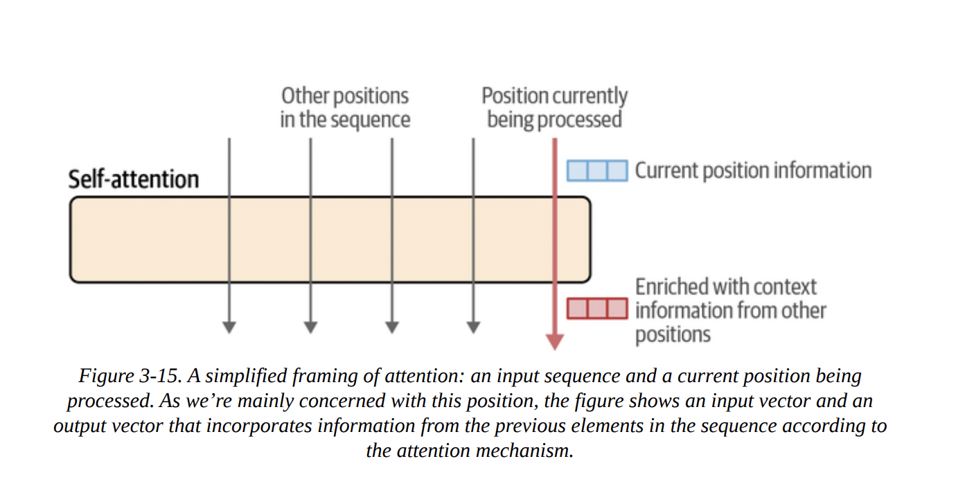
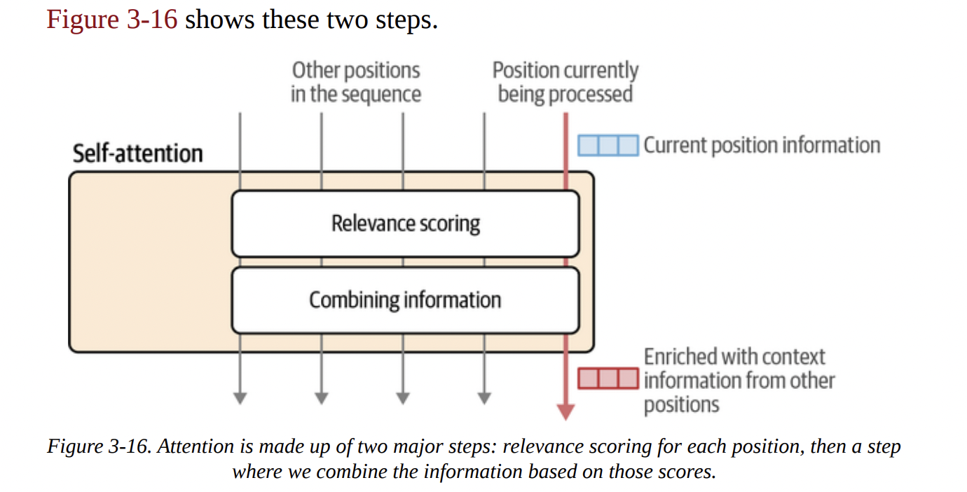
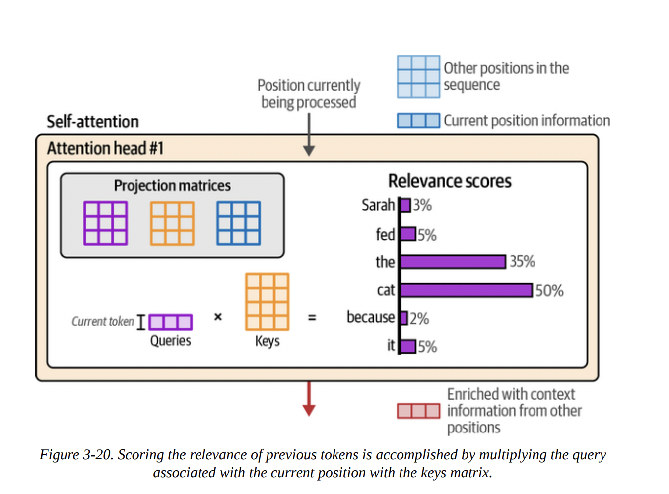
- Relevance Scoring: For the current token we’re processing, calculate a score for every other token in the context that tells us how relevant it is.
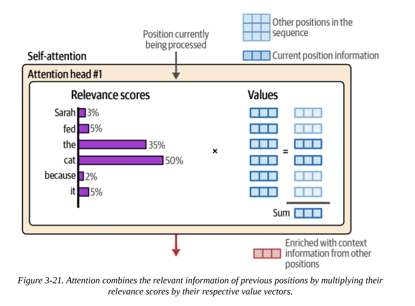
- Combining Information: Create a new vector for the current token by taking a weighted sum of all the other token vectors, using the relevance scores as weights.
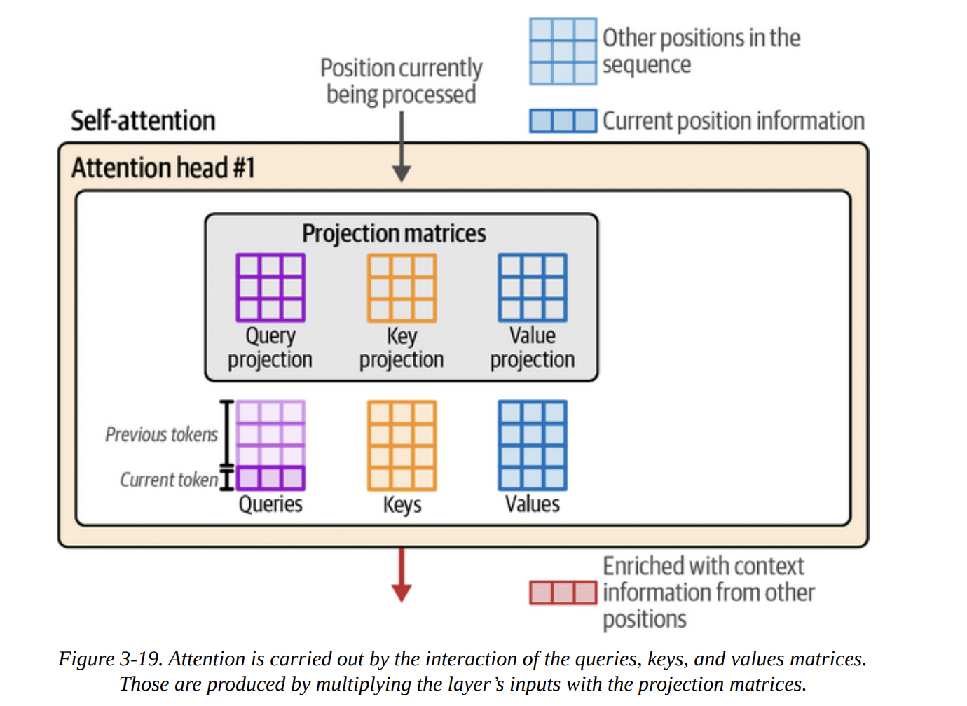
To do this, we use the famous Query, Key, Value (QKV) model. Imagine this:
- You are the Query: the current token, asking for information.
- Every other token is a Key: a label for the information it holds.
- Every other token also has a Value: the actual information it holds.
The process, shown in Figures 3-18 through 3-21, is:
- Projection: The input vectors are multiplied by three separate weight matrices (learned during training) to create the Q, K, and V vectors for each token (see Figure 3-19).
- Scoring: You (the Query) compare yourself to every other token’s Key. This is done with a dot product:
Q · K^T. The result is a set of raw scores. After a softmax function, these become the attention scores (our relevance scores), summing to 1 (see Figure 3-20). - Combining: These scores are then used to create a weighted sum of all the Value vectors. A token with a high score contributes more of its Value to the final output. The result is the new, context-enriched vector for the current position (see Figure 3-21).
Let me draw this core QKV logic with a diagram to make it even clearer.
graph TD
    subgraph Input Vectors for each token
        direction LR
        I1(Token 1 Vector)
        I2(Token 2 Vector)
        I3(Token 3 Vector)
    end

    subgraph Projection Matrices
        direction LR
        W_Q(Query Matrix Wq)
        W_K(Key Matrix Wk)
        W_V(Value Matrix Wv)
    end

    subgraph "Step 1: Create Q, K, V vectors"
        direction LR
        Q1(Q1)
        K1(K1)
        V1(V1)
        Q2(Q2)
        K2(K2)
        V2(V2)
        Q3(Q3)
        K3(K3)
        V3(V3)
    end

    I1 -- x Wq --> Q1
    I1 -- x Wk --> K1
    I1 -- x Wv --> V1
    I2 -- x Wq --> Q2
    I2 -- x Wk --> K2
    I2 -- x Wv --> V2
    I3 -- x Wq --> Q3
    I3 -- x Wk --> K3
    I3 -- x Wv --> V3

    subgraph "Step 2: Score (e.g., for Token 3)"
        S1(Score_3_1 = Q3 • K1)
        S2(Score_3_2 = Q3 • K2)
        S3(Score_3_3 = Q3 • K3)
        SM(Softmax)
        S1 & S2 & S3 --> SM
    end

    subgraph "Step 3: Combine based on Scores"
        O3(Output Vector for Token 3)
    end

    SM -- Weights --> O3
    V1 & V2 & V3 -- Vectors to be weighted --> O3

    linkStyle 11 stroke:#ff0000,stroke-width:2px;
    linkStyle 12 stroke:#0000ff,stroke-width:2px;
    linkStyle 13 stroke:#00ff00,stroke-width:2px;
This entire QKV calculation is done in parallel inside multiple attention heads, allowing the model to focus on different kinds of relationships (e.g., one head for syntax, another for semantics) simultaneously.
Recent Improvements to the Transformer Architecture
The original Transformer was from 2017. The field has evolved. Let’s cover the modern enhancements mentioned in the book.
More Efficient Attention
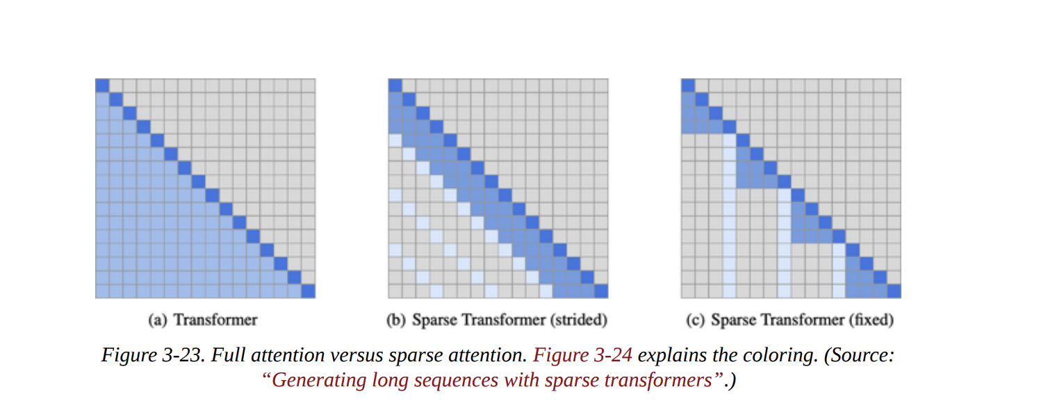
As models got bigger, the N^2 complexity of full attention became a bottleneck.
- Local/Sparse Attention: As shown in Figure 3-23, instead of attending to all previous tokens, a token might only attend to a small, local window or a “strided” pattern. This is much faster but can lose global context. GPT-3 cleverly alternates between full and sparse attention layers.
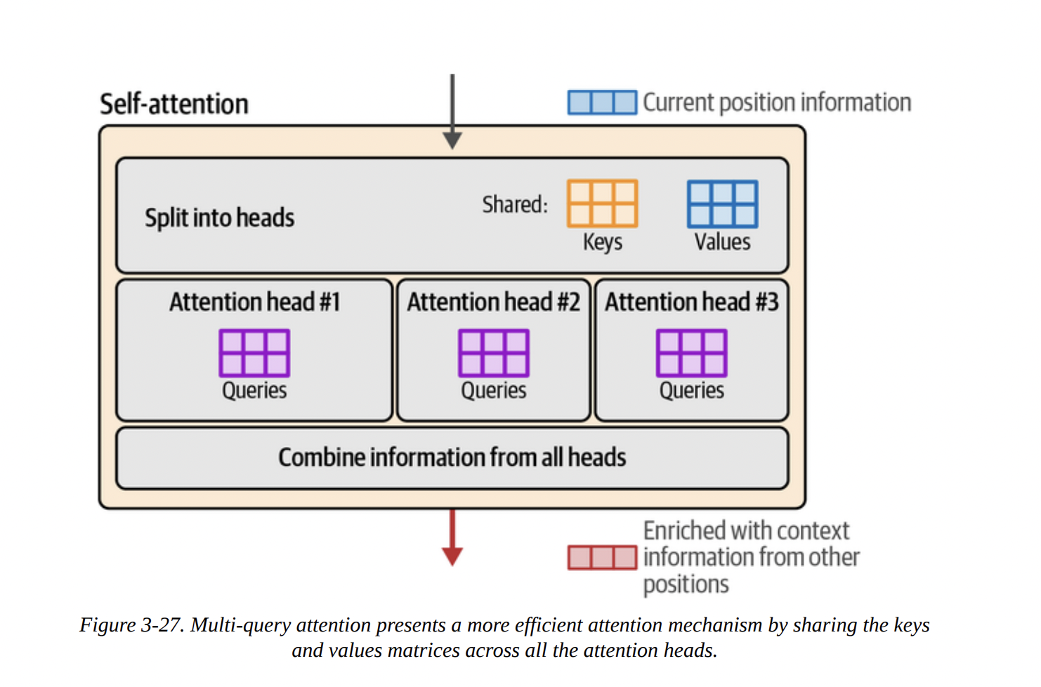
- Multi-Query and Grouped-Query Attention (MQA/GQA): Full multi-head attention (MHA) has separate K and V matrices for every head. This uses a lot of memory for the KV Cache.
- MQA: A major optimization where all heads share a single Key and Value matrix (see Figure 3-27). This drastically reduces the KV cache size but can hurt model quality.
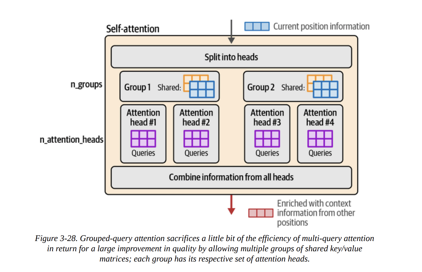
- GQA: A happy medium. Heads are divided into groups, and heads within a group share K and V matrices (see Figure 3-28). This is used by models like Llama 2 and Phi-3, offering a great balance of speed and quality.
Here’s a diagram illustrating the evolution from MHA to GQA.
graph TD
    subgraph "Multi-Head Attention (MHA)"
        H1_MHA("Head 1 <br/> Q1, K1, V1")
        H2_MHA("Head 2 <br/> Q2, K2, V2")
        H3_MHA("Head 3 <br/> Q3, K3, V3")
        H4_MHA("Head 4 <br/> Q4, K4, V4")
    end

    subgraph "Multi-Query Attention (MQA)"
        H1_MQA("Head 1 <br/> Q1") --> KV_MQA("Shared K, V")
        H2_MQA("Head 2 <br/> Q2") --> KV_MQA
        H3_MQA("Head 3 <br/> Q3") --> KV_MQA
        H4_MQA("Head 4 <br/> Q4") --> KV_MQA
    end

    subgraph "Grouped-Query Attention (GQA)"
        subgraph "Group 1"
            H1_GQA("Head 1 <br/> Q1") --> KV1_GQA("Shared K1, V1")
            H2_GQA("Head 2 <br/> Q2") --> KV1_GQA
        end
        subgraph "Group 2"
            H3_GQA("Head 3 <br/> Q3") --> KV2_GQA("Shared K2, V2")
            H4_GQA("Head 4 <br/> Q4") --> KV2_GQA
        end
    end

    H1_MHA -.-> H1_MQA
    H1_MQA -.-> H1_GQA
- FlashAttention: Not an algorithmic change, but a brilliant re-implementation. It optimizes the way Q, K, and V matrices are moved between the GPU’s fast SRAM and slower HBM, avoiding bottlenecks and providing massive speedups for both training and inference.
The Modern Transformer Block
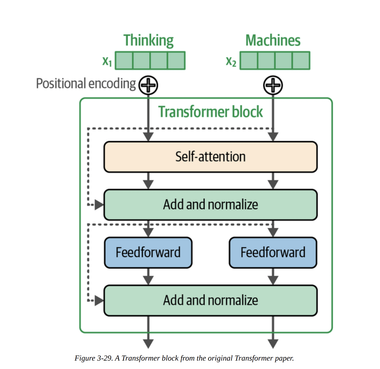
Figure 3-29 shows the original block, which used “post-normalization” (Add & Norm after the sub-layer). Figure 3-30 shows a modern block, like in Llama or Phi-3, with key differences:
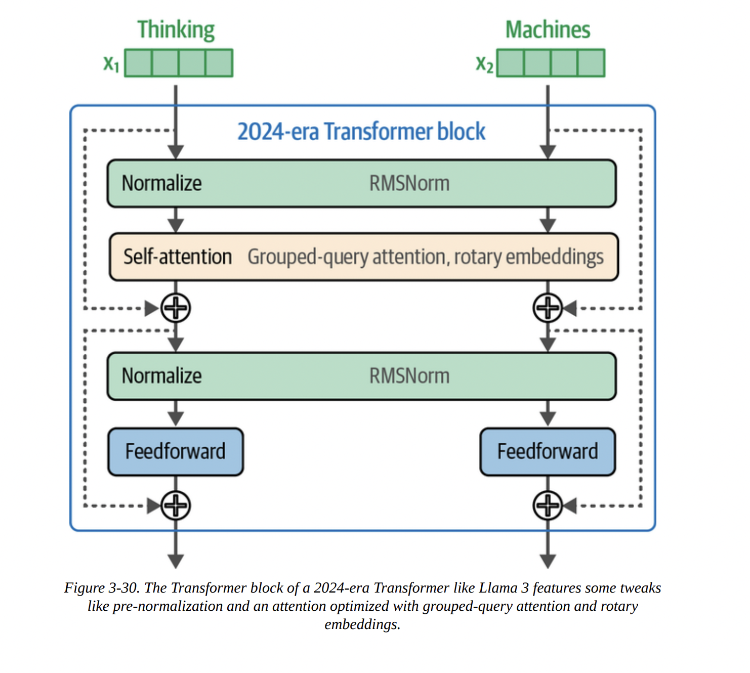
- Pre-Normalization: The normalization layer (like RMSNorm) is applied before the attention and FFN layers. This leads to more stable training.
- RMSNorm: A simpler, faster alternative to the original LayerNorm.
- SwiGLU: A more advanced activation function for the FFN, replacing the original ReLU.
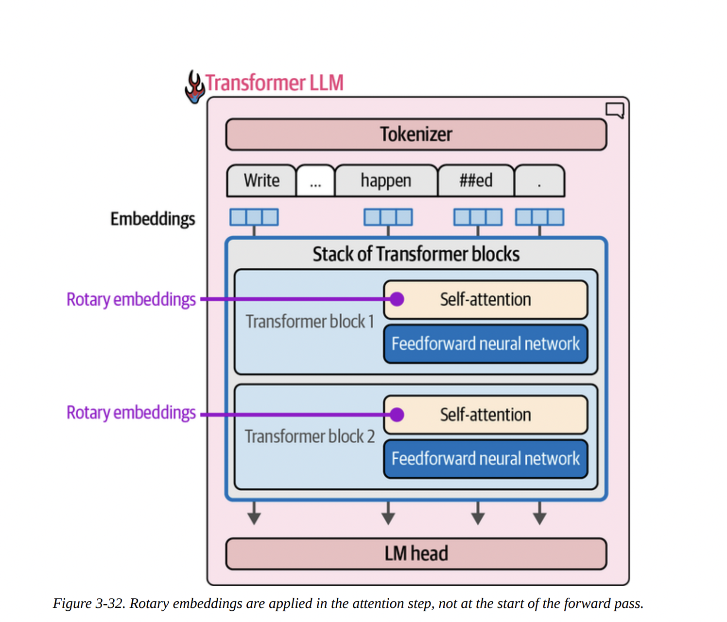
- Rotary Positional Embeddings (RoPE).
Positional Embeddings (RoPE)
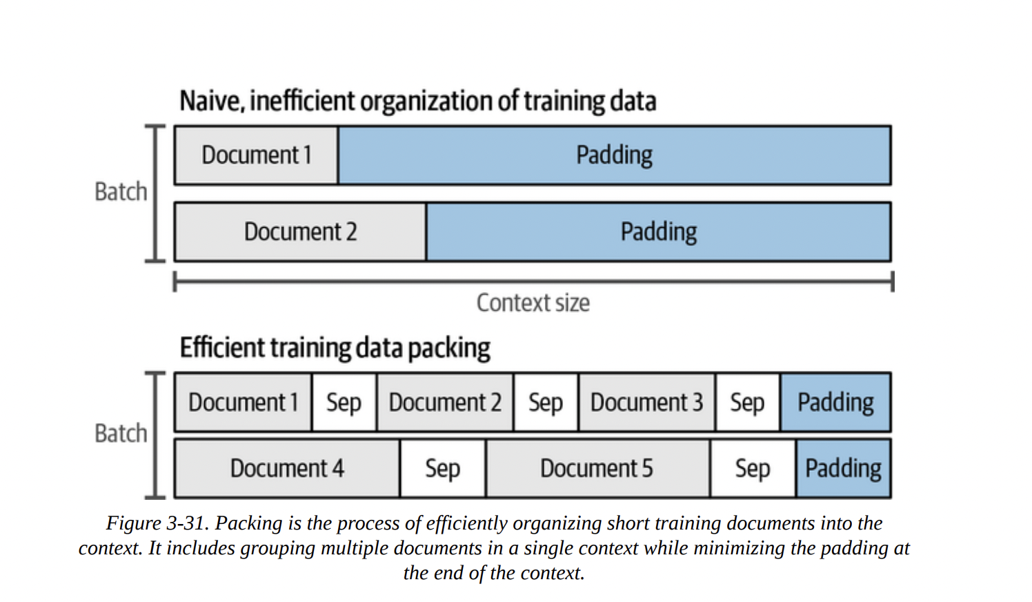
Transformers are inherently “bags of vectors”; they don’t know the order of tokens. We need to inject positional information. The old way was to add a positional embedding to the token embedding at the very beginning. But this is inflexible, especially when “packing” multiple documents into one context, as shown in Figure 3-31.
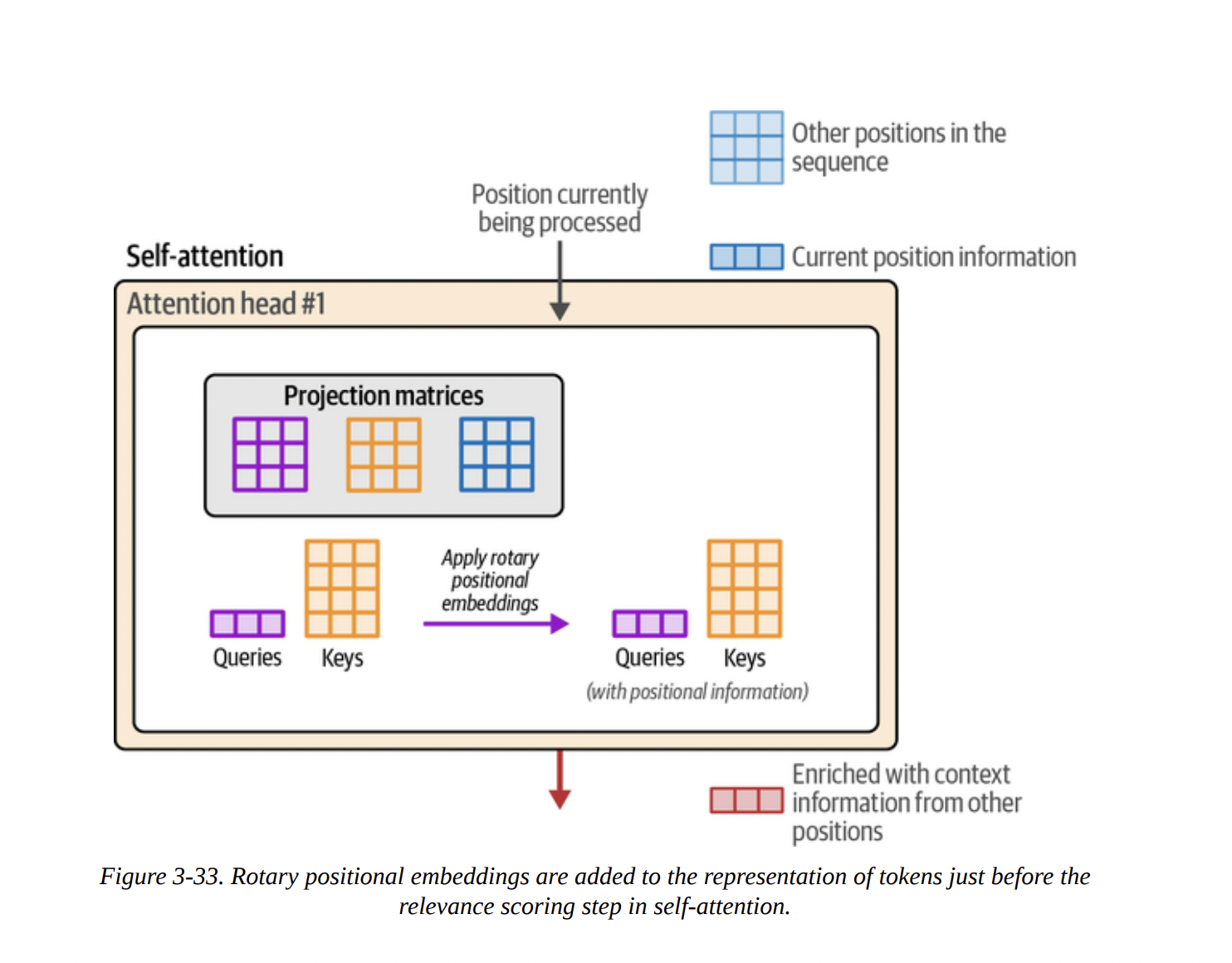
RoPE is a clever solution. Instead of adding a vector, it rotates the Query and Key vectors based on their absolute position. This is done inside the attention layer, just before the Q · K multiplication (as shown in Figures 3-32 and 3-33). This method has proven to be incredibly effective, as it elegantly encodes both absolute and relative position information.
Summary
And that brings us to the end of a very dense but crucial chapter. We have peered deep inside the Transformer.
We’ve seen that generation is an autoregressive, token-by-token loop. We dissected the forward pass into its three main components: the tokenizer, the stack of Transformer blocks, and the LM head. We learned that this process is parallelized across tokens and that the KV cache is a vital optimization to speed it up.
Most importantly, we opened up the Transformer block itself and demystified its two workhorses: the feedforward network for storing knowledge and the attention mechanism for incorporating context. We went deep into the QKV model of attention and looked at modern improvements like GQA and FlashAttention. Finally, we touched on architectural tweaks like pre-normalization and the powerful Rotary Positional Embeddings (RoPE).