Chapter 4: Text Classification

As the book opens, it states a simple goal: classification is about assigning a label or class to some input text. This is a cornerstone of NLP. Think about it:

• Is this email spam or not? (Spam detection)
• Is this customer review positive, negative, or neutral? (Sentiment analysis)
• Is this news article about sports, politics, or technology? (Topic classification)

Figure 4-1 gives us the high-level picture: text goes in, the model does its thing, and a category comes out.

The real meat of this chapter, and what makes it so relevant today, is that we can tackle this problem with two different families of models, as shown in Figure 4-2:

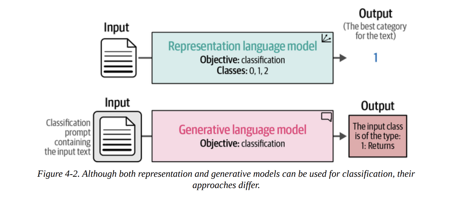
1. Representation Models (Encoder-style, like BERT): These models are designed to understand text and output numerical representations. For classification, they typically output a final class ID (e.g., 1 for “Returns”).
2. Generative Models (Decoder-style, like GPT, or Encoder-Decoder like T5): These models are designed to generate text. To get a class out of them, we have to cleverly prompt them to output the text of the label (e.g., the string “Returns”).

We will explore both paths. But first, we need a problem to solve and data to solve it with.

The Sentiment of Movie Reviews

The book wisely chooses a classic and intuitive dataset: rotten_tomatoes. The task is simple: determine if a movie review is positive or negative.

Let’s load the data using the datasets library from Hugging Face. This is a standard workflow you’ll use constantly.

from datasets import load_dataset

# Load our data
data = load_dataset("rotten_tomatoes")

When we inspect data, we get the following structure:

DatasetDict({
    train: Dataset({
        features: ['text', 'label'],
        num_rows: 8530
    })
    validation: Dataset({
        features: ['text', 'label'],
        num_rows: 1066
    })
    test: Dataset({
        features: ['text', 'label'],
        num_rows: 1066
    })
})

This is great. The data is already split for us into train, validation, and test sets. As good practitioners, we’ll use the train set for any training, and the test set for our final evaluation. The validation set is there if we need to do hyperparameter tuning, to avoid “peeking” at the final test set.

Let’s look at a couple of examples. The label 1 is positive, and 0 is negative.

# data["train"][0, -1]
{'text': ["the rock is destined to be the 21st century's new conan...", 
          'things really get weird , though not particularly scary...'], 
 'label': [1, 0]}

The task is clear. Now, let’s see how our first family of models tackles it.

Text Classification with Representation Models

As we discussed in previous chapters, representation models like BERT are phenomenal at understanding language. They are typically pre-trained on a massive corpus of text (like Wikipedia) to learn the nuances of language. Then, they are fine-tuned for specific tasks.

Figure 4-3 shows this beautifully. We start with a base foundation model (like BERT). We can then fine-tune it for a specific task like classification, creating a task-specific model. Alternatively, we can fine-tune it to produce high-quality general-purpose embeddings.

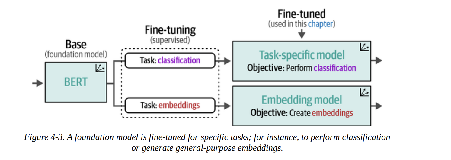
In this chapter, we’re not doing the fine-tuning ourselves (we’ll save that for Chapters 10 and 11). Instead, we’ll use models that others have already fine-tuned for us. Figure 4-4 shows our two strategies:

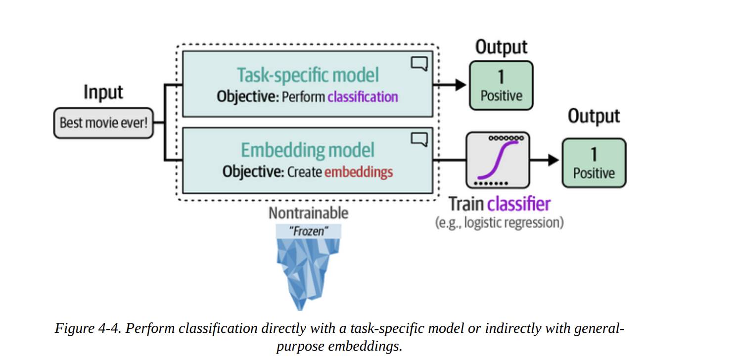
1. Directly use a task-specific model that outputs a classification.
2. Use an embedding model to convert text to vectors, and then train a simple, classical classifier (like logistic regression) on those vectors.

Model Selection

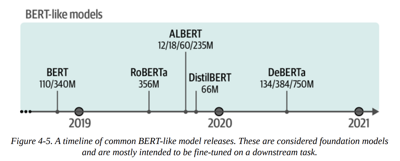
The Hugging Face Hub is vast. Figure 4-5 gives a glimpse into the timeline of just the BERT-like models. How do we choose? The book gives some solid baselines like bert-base-model or roberta-base-model.

For our first approach, we’ll use a task-specific model: cardiffnlp/twitter-roberta-base-sentiment-latest. This is a RoBERTa model that was fine-tuned for sentiment on Tweets. It’s an interesting choice because we’re testing how well it generalizes from the short, informal language of Twitter to our movie review dataset.

Using a Task-Specific Model

We can use the pipeline abstraction from transformers, which makes inference incredibly simple.

from transformers import pipeline

# Path to our HF model
model_path = "cardiffnlp/twitter-roberta-base-sentiment-latest"

# Load model into pipeline
pipe = pipeline(
    "text-classification", # We specify the task
    model=model_path,
    tokenizer=model_path, # Good practice to be explicit
    return_all_scores=True,
    device="cuda:0"
)

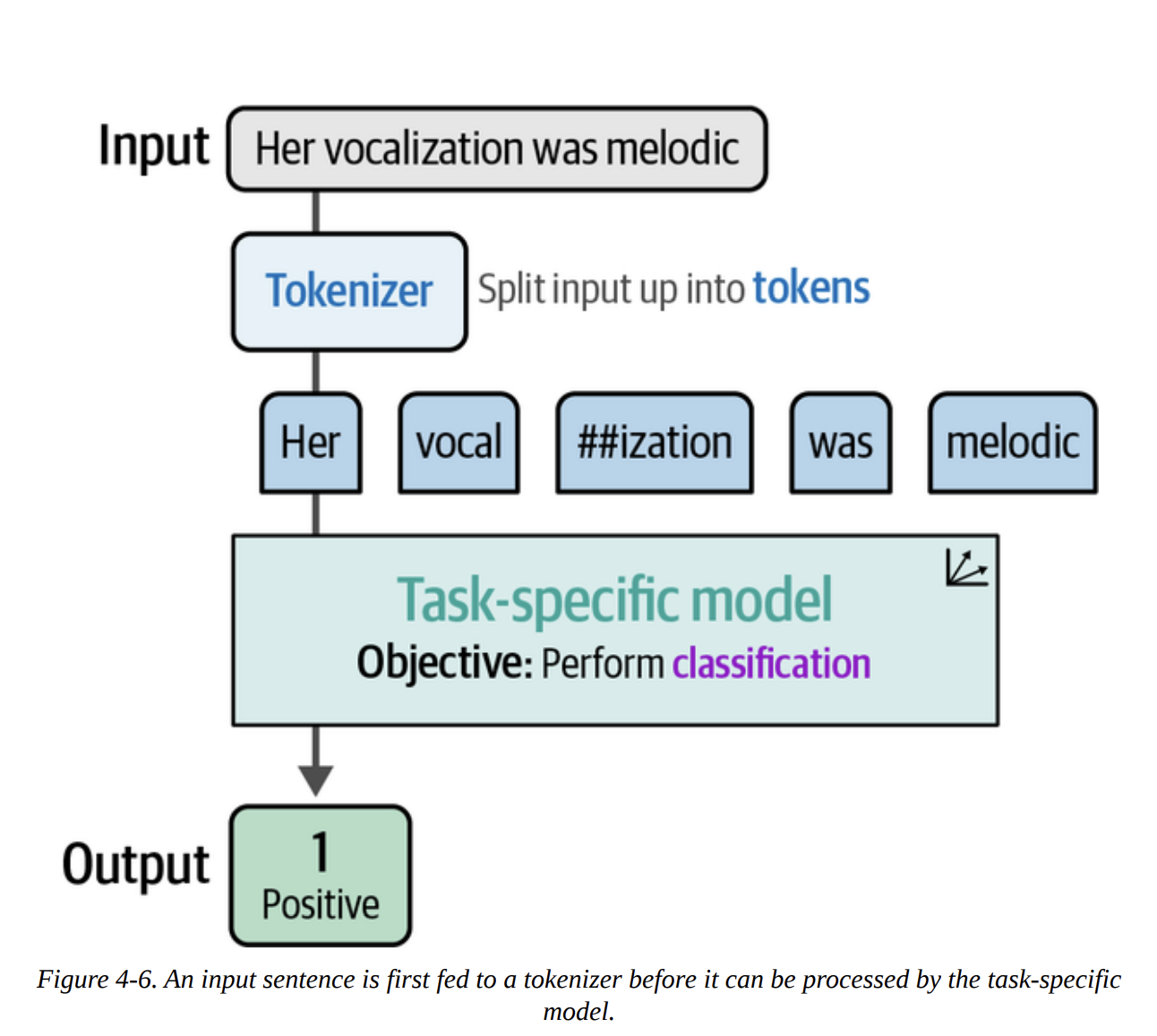
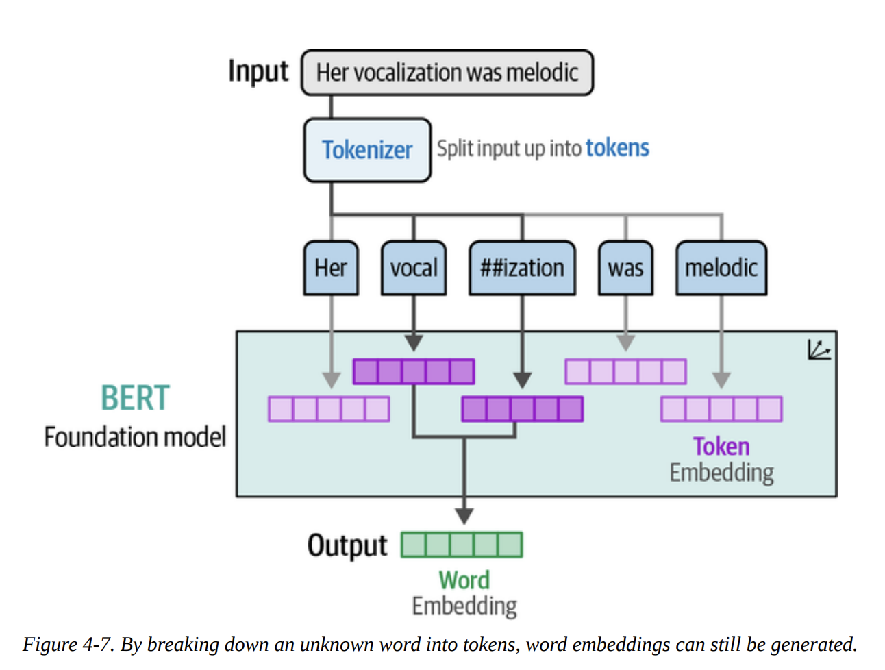
As Figure 4-6 illustrates, when we pass text to this pipeline, it first gets tokenized, then processed by the model, which outputs the classification. The power of subword tokenization, as shown in Figure 4-7, means the model can handle words it’s never seen before by breaking them down into known sub-parts.

Now, let’s run this pipeline on our entire test set and evaluate it.

import numpy as np
from tqdm import tqdm
from transformers.pipelines.pt_utils import KeyDataset

# Run inference
y_pred = []
# The model outputs scores for 'Negative', 'Neutral', 'Positive'
# We are interested in Negative (index 0) vs Positive (index 2)
for output in tqdm(pipe(KeyDataset(data["test"], "text")), total=len(data["test"])):
    negative_score = output[0]["score"]
    positive_score = output[2]["score"]
    assignment = np.argmax([negative_score, positive_score]) # 0 for negative, 1 for positive
    y_pred.append(assignment)

Now we have our predictions (y_pred) and the true labels (data["test"]["label"]). Let’s evaluate. The book provides a handy function.

from sklearn.metrics import classification_report

def evaluate_performance(y_true, y_pred):
    """Create and print the classification report"""
    performance = classification_report(
        y_true, y_pred, target_names=["Negative Review", "Positive Review"]
    )
    print(performance)

evaluate_performance(data["test"]["label"], y_pred)

This gives us the classification report:

               precision    recall  f1-score   support

Negative Review       0.76      0.88      0.81       533
Positive Review       0.86      0.72      0.78       533

       accuracy                           0.80      1066
      macro avg       0.81      0.80      0.80      1066
   weighted avg       0.81      0.80      0.80      1066

To really understand this, let’s quickly break down the key metrics, which the book visualizes in Figure 4-9:

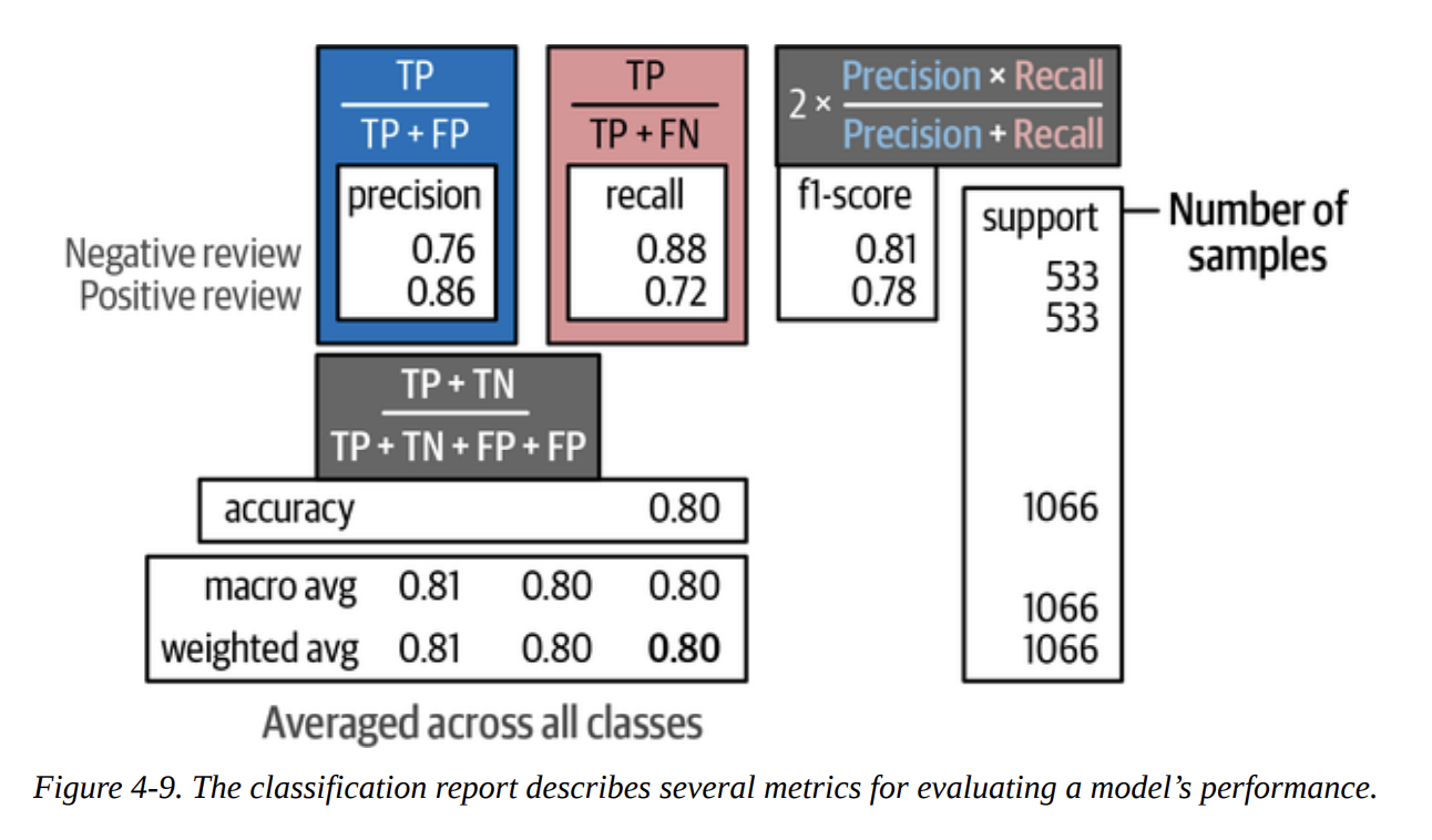
• Precision: Of all the times we predicted “Positive”, how many were actually positive? (Here, 86%). This is about not making false positive mistakes.
• Recall: Of all the reviews that were actually “Positive”, how many did we find? (Here, 72%). This is about not missing any actual positives.
• F1-score: The harmonic mean of precision and recall. It’s a single number that balances both concerns.
• Weighted Avg F1-score: 0.80. This is a very respectable score, especially considering the model was trained on Twitter data, not movie reviews! This shows the power of pre-training.

Classification Tasks That Leverage Embeddings

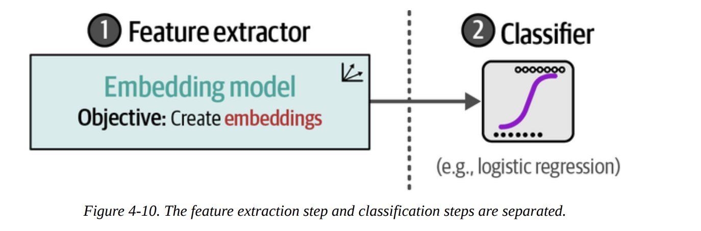
What if a ready-made, task-specific model doesn’t exist for our problem? Do we have to do a full, expensive fine-tuning run? No!

This is where the second strategy from Figure 4-4 comes in. We can use a model that’s great at creating general-purpose embeddings. This acts as a powerful feature extractor. Then, we can train a very simple, lightweight classifier on these features. The process, shown in Figure 4-10, separates feature extraction from classification.

For this, we’ll use the sentence-transformers/all-mpnet-base-v2 model, a top performer on embedding benchmarks.

Step 1: Create Embeddings (as in Figure 4-11)

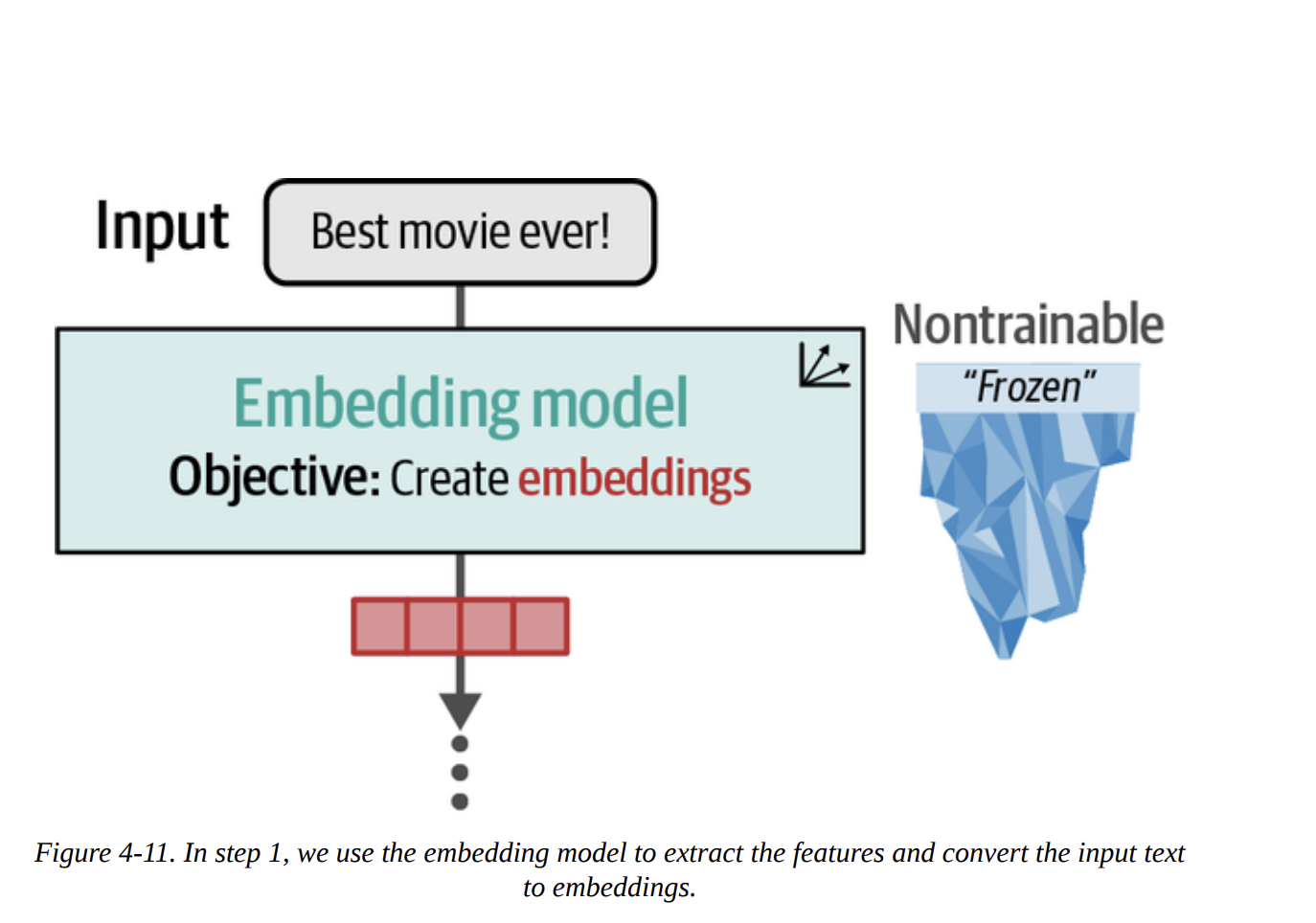
from sentence_transformers import SentenceTransformer

# Load model
model = SentenceTransformer("sentence-transformers/all-mpnet-base-v2")

# Convert text to embeddings
train_embeddings = model.encode(data["train"]["text"], show_progress_bar=True)
test_embeddings = model.encode(data["test"]["text"], show_progress_bar=True)

The shape of train_embeddings will be (8530, 768), meaning we have a 768-dimensional vector for each of our 8,530 training reviews.

Step 2: Train a Classifier (as in Figure 4-12)

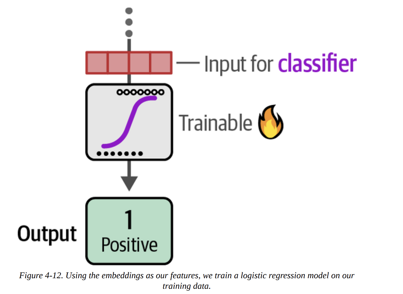
Now we treat this like a classic ML problem. The embeddings are our features (X), and the labels are our targets (y).

from sklearn.linear_model import LogisticRegression

# Train a logistic regression on our train embeddings
clf = LogisticRegression(random_state=42)
clf.fit(train_embeddings, data["train"]["label"])

# Predict previously unseen instances
y_pred = clf.predict(test_embeddings)
evaluate_performance(data["test"]["label"], y_pred)

The result:

               precision    recall  f1-score   support

Negative Review       0.85      0.86      0.85       533
Positive Review       0.86      0.85      0.85       533
...
   weighted avg       0.85      0.85      0.85      1066

An F1-score of 0.85! We actually improved our performance by using general-purpose embeddings and a simple classifier. This is a powerful and flexible technique.

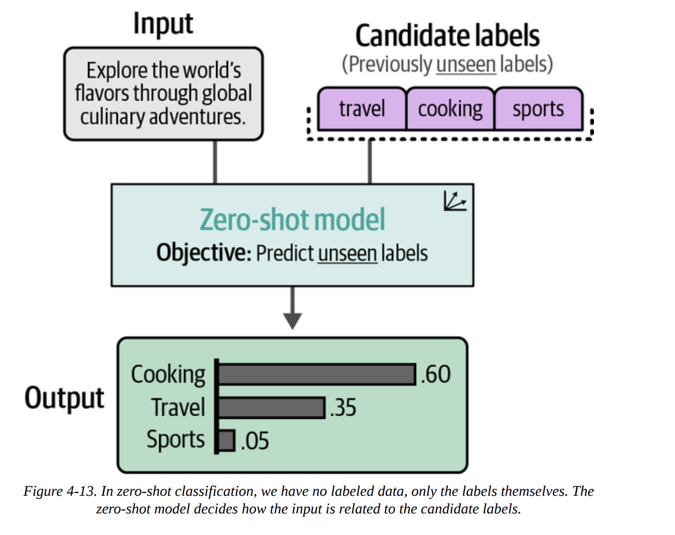
What If We Do Not Have Labeled Data?

This is where things get really interesting. What if we don’t have any labeled data? This is called zero-shot classification. The core idea, shown in Figure 4-13, is to classify text against a set of candidate labels that the model has never been explicitly trained on.

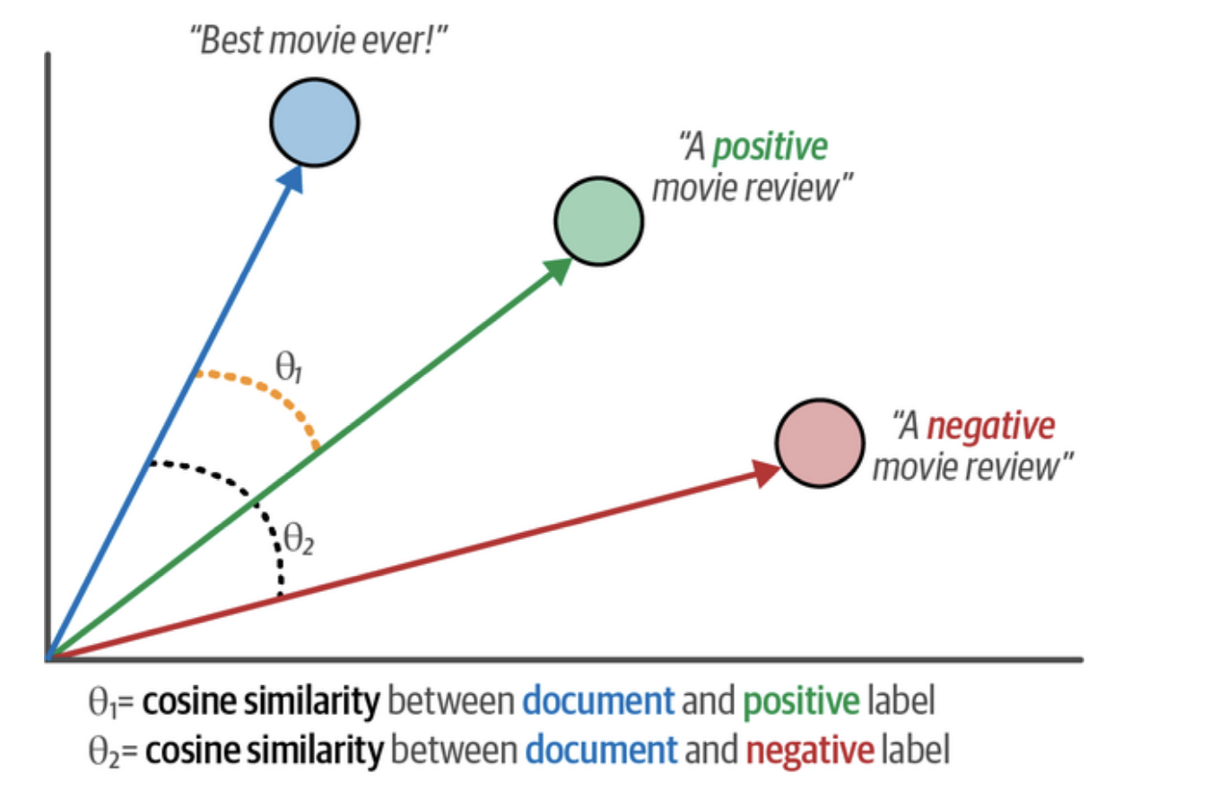
How do we do this with embeddings? The book shows a brilliant trick. Instead of using abstract labels like 0 and 1, we create descriptive sentences for our labels.

• 0 becomes "A negative movie review"
• 1 becomes "A positive movie review"

Then, as Figure 4-14 illustrates, we embed both our documents and our descriptive labels into the same vector space.

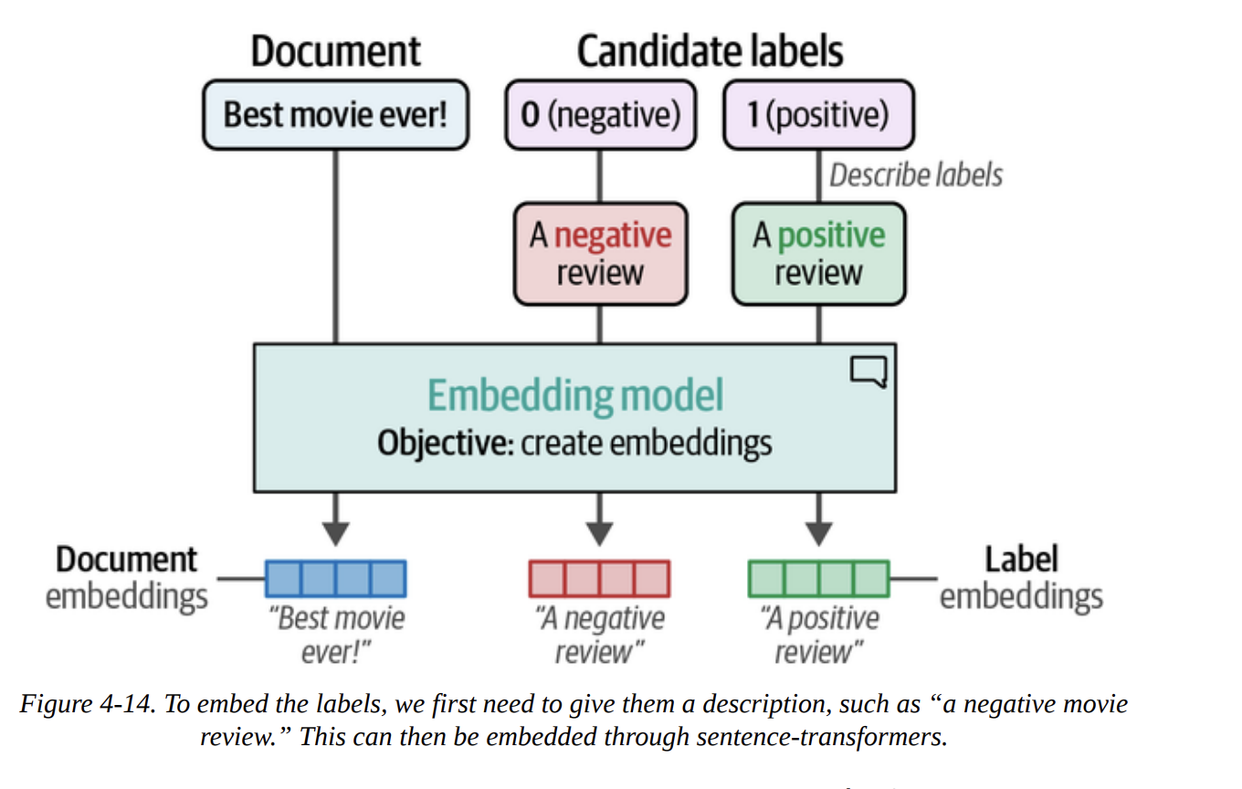
# Create embeddings for our labels
label_embeddings = model.encode(["A negative review", "A positive review"])

Now, for each document embedding, we can calculate its cosine similarity to each of the label embeddings. Cosine similarity measures the angle between two vectors, as visualized in Figure 4-15. A smaller angle (higher similarity) means they are closer in meaning. We simply assign the label with the highest similarity.

from sklearn.metrics.pairwise import cosine_similarity

# Find the best matching label for each document
sim_matrix = cosine_similarity(test_embeddings, label_embeddings)
y_pred = np.argmax(sim_matrix, axis=1)

evaluate_performance(data["test"]["label"], y_pred)

The result:

               precision    recall  f1-score   support

Negative Review       0.78      0.77      0.78       533
Positive Review       0.77      0.79      0.78       533
...
   weighted avg       0.78      0.78      0.78      1066

An F1-score of 0.78! This is astonishing. Without a single labeled example, just by describing our labels, we achieved a result that’s almost as good as our fully supervised models. This is a testament to the power of high-quality embeddings.

Text Classification with Generative Models

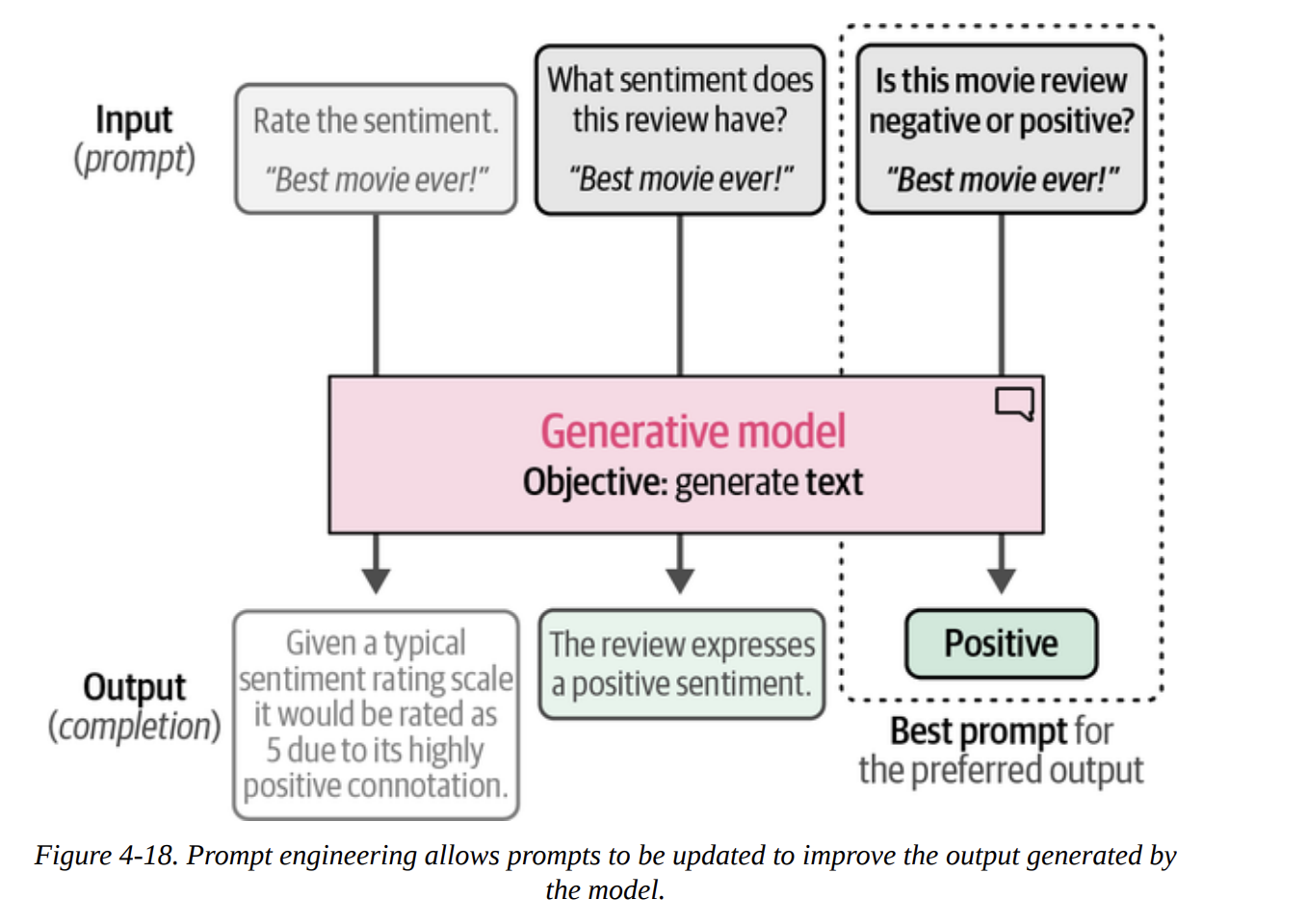
Now we switch to the other family of models. These are sequence-to-sequence models. They don’t output a class ID; they output text. To make them classify, we need to guide them with an instruction, or prompt. This iterative process of refining the instruction is called prompt engineering, shown beautifully in Figure 4-18.

Using the Text-to-Text Transfer Transformer (Flan-T5)

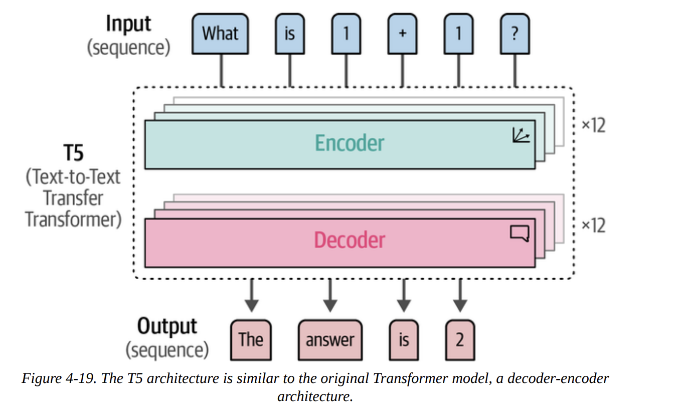
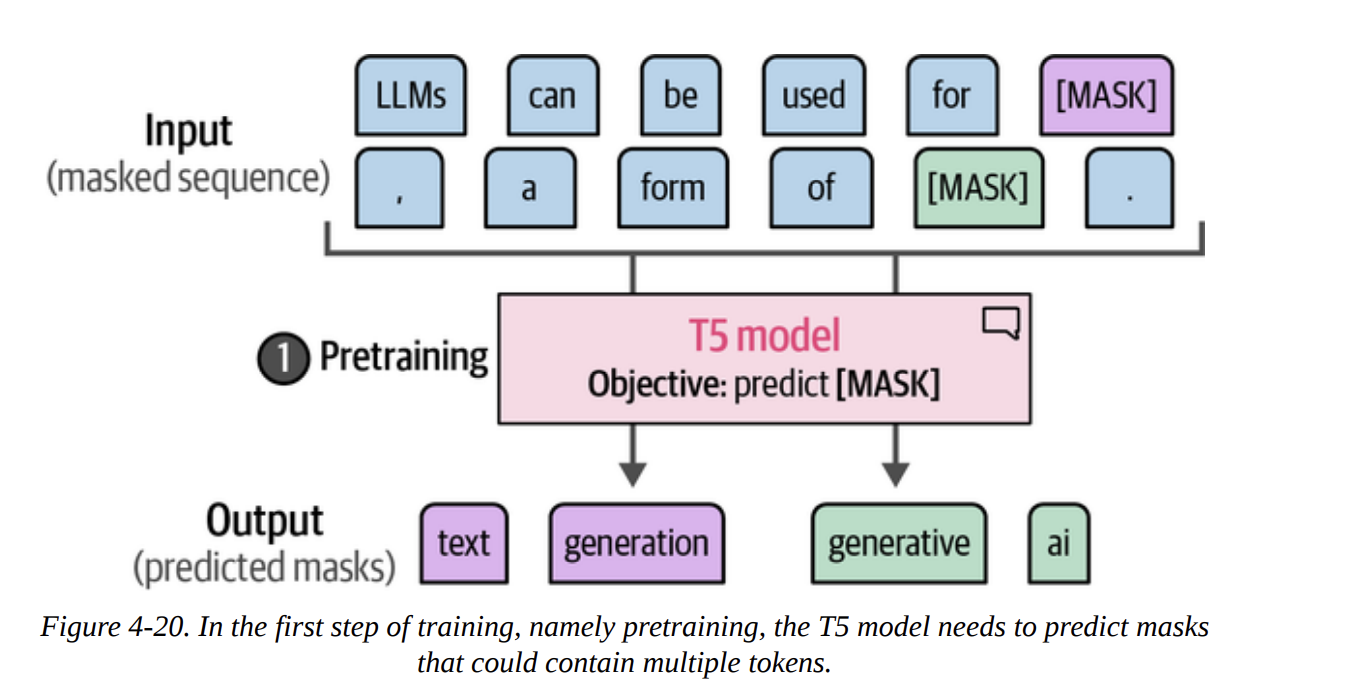
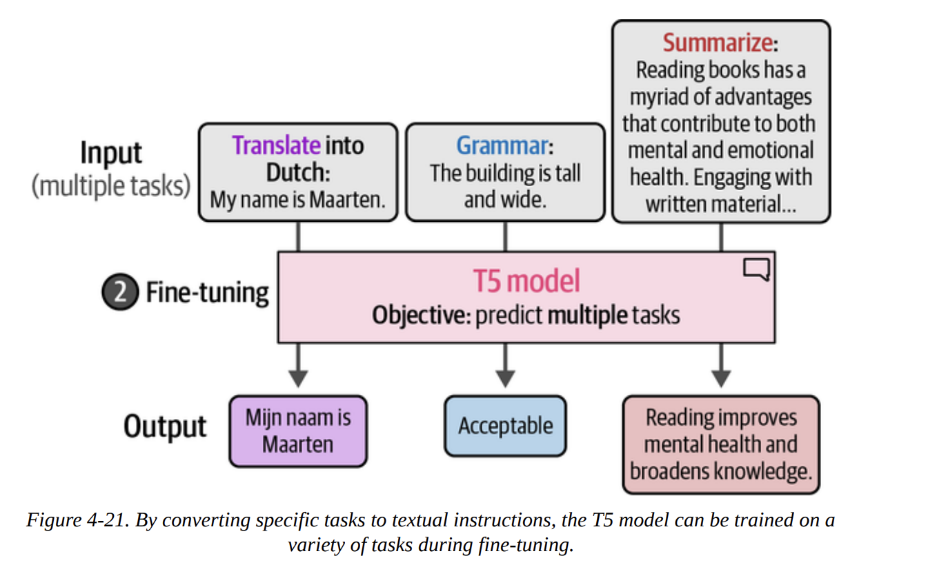
First, we’ll look at an open-source generative model. T5 is an encoder-decoder model (Figure 4-19). Its big innovation was framing every NLP task as a text-to-text problem during its fine-tuning phase (Figures 4-20 and 4-21). The Flan-T5 models were further fine-tuned on many instruction-based tasks, making them great at following prompts.

Let’s load the small version.

pipe = pipeline(
    "text2text-generation",
    model="google/flan-t5-small",
    device="cuda:0"
)

We can’t just feed it the review. We have to create a prompt. Let’s prefix every review with a question.

# Prepare our data
prompt = "Is the following sentence positive or negative? "
data = data.map(lambda example: {"t5": prompt + example['text']})

Now we run inference, but we have to parse the text output.

y_pred = []
for output in tqdm(pipe(KeyDataset(data["test"], "t5")), total=len(data["test"])):
    text = output[0]["generated_text"]
    y_pred.append(0 if text.lower() == "negative" else 1)

The result is an F1-score of 0.84. This is very strong and shows that prompting generative models is a highly effective classification strategy.

ChatGPT for Classification

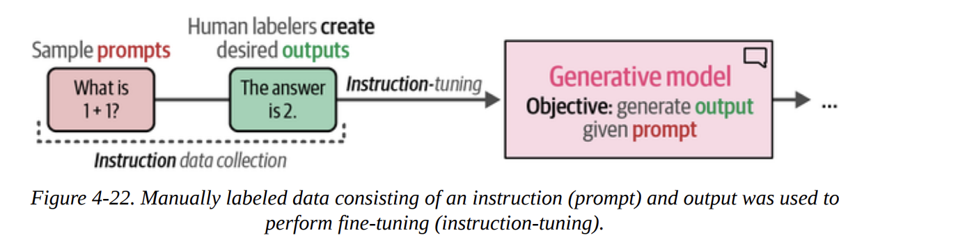
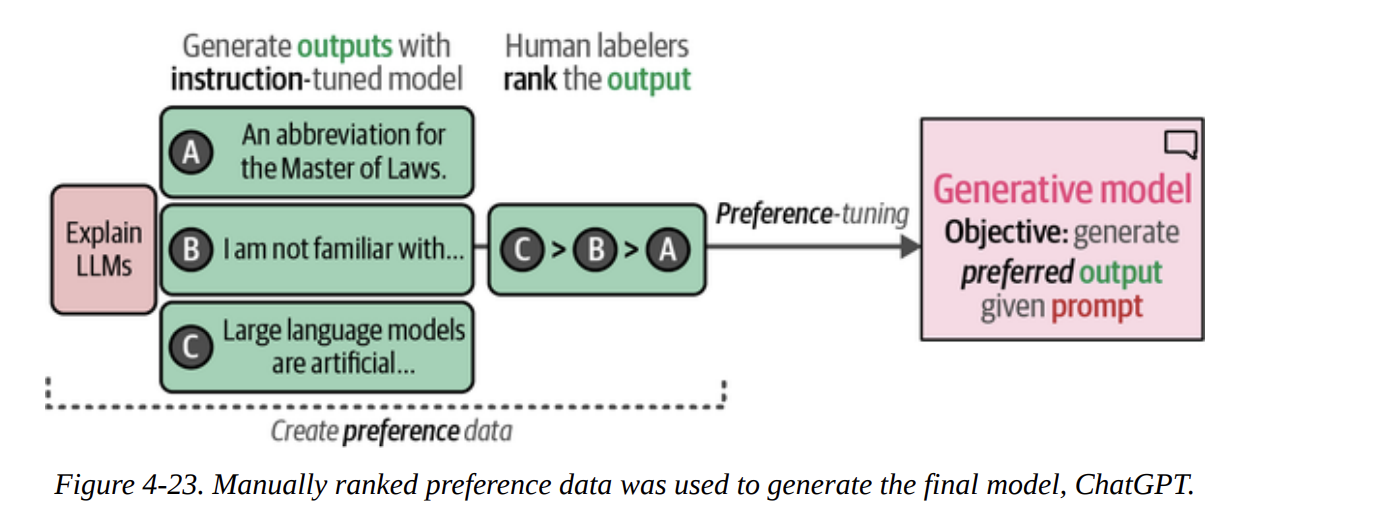
Finally, we’ll look at a closed-source, decoder-only model: ChatGPT. We access it via an API. The book explains its training process, including instruction tuning (Figure 4-22) and the crucial preference tuning (RLHF) step (Figure 4-23).

First, we set up our client.

import openai
# You need to get your own key from OpenAI
client = openai.OpenAI(api_key="YOUR_KEY_HERE")

We then write a much more detailed prompt, telling the model exactly what to do and what format to return. This is a powerful form of prompt engineering.

prompt = """Predict whether the following document is a positive or negative movie review:

[DOCUMENT]

If it is positive return 1 and if it is negative return 0. Do not give any other answers."""

# Example call
document = "unpretentious , charming , quirky , original"
# chatgpt_generation(prompt, document) # a helper function defined in the book

After running this on the test set and converting the string outputs ("1" or "0") to integers, we get the evaluation:

               precision    recall  f1-score   support

Negative Review       0.87      0.97      0.92       533
Positive Review       0.96      0.86      0.91       533
...
   weighted avg       0.92      0.91      0.91      1066

An F1-score of 0.91! A remarkable performance. However, the book makes a critical point for any data scientist: with a closed-source model, we don’t know its training data. It’s possible the rotten_tomatoes dataset was part of its training, which would make this evaluation invalid. This is a key consideration when working with proprietary models.

Summary

This chapter was our first deep dive into a practical application, and what a journey it was.

We saw that text classification can be tackled with two families of models.

• Representation models are excellent, either used directly as fine-tuned classifiers (F1=0.80) or as powerful feature extractors for classical ML models (F1=0.85). We even saw their incredible flexibility with zero-shot classification via cosine similarity (F1=0.78).
• Generative models are also formidable classifiers when guided by good prompt engineering. We saw strong results from an open-source encoder-decoder model like Flan-T5 (F1=0.84) and state-of-the-art performance from a closed-source model like ChatGPT (F1=0.91), with important caveats.