Chapter 5: Text Clustering and Topic Modeling

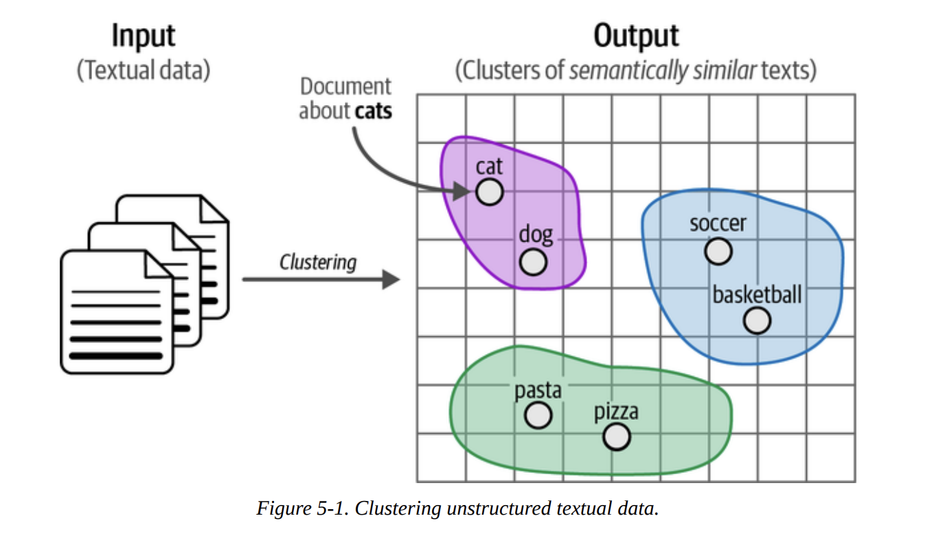
The goal is simple but profound: to automatically group similar texts together based on their meaning. As Figure 5-1 illustrates, we start with a heap of unstructured documents and aim to produce clusters where documents about “pets” are in one group, “sports” in another, and “food” in a third. This is immensely powerful for quick data exploration, finding unexpected themes, or even pre-categorizing data for later supervised tasks.

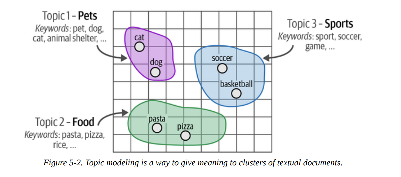
As we move from clustering to topic modeling, our goal refines slightly. We don’t just want the groups; we want a meaningful description for each group. Figure 5-2 shows this transition: the “pets” cluster is described by keywords like pet, dog, cat, etc. This gives us a human-understandable label for the abstract group.

This chapter is a masterclass in combining different types of models. We’ll see how modern embedding models (encoder-only), classical NLP techniques (bag-of-words), and even powerful generative models (decoder-only) can be chained together in a pipeline to create something truly impressive.

ArXiv’s Articles: Computation and Language

To make this tangible, we need a dataset. The book chooses a fantastic one: a collection of 44,949 abstracts from ArXiv’s “Computation and Language” (cs.CL) section. This is perfect because it’s real, complex data, and it’s relevant to our field.

Let’s start by loading the data, just as the book does.

# Load data from Hugging Face
from datasets import load_dataset

dataset = load_dataset("maartengr/arxiv_nlp")["train"]

# Extract metadata
abstracts = dataset["abstracts"]
titles = dataset["titles"]

We now have our collection of abstracts ready. Our mission is to find the hidden topics within them.

A Common Pipeline for Text Clustering

The book lays out a very common and effective three-step pipeline for modern text clustering. This is our foundational recipe:

1. Embed: Convert all documents into numerical vectors (embeddings).
2. Reduce: Lower the dimensionality of these embeddings.
3. Cluster: Group the low-dimensional points together.

Let’s walk through each step.

Embedding Documents

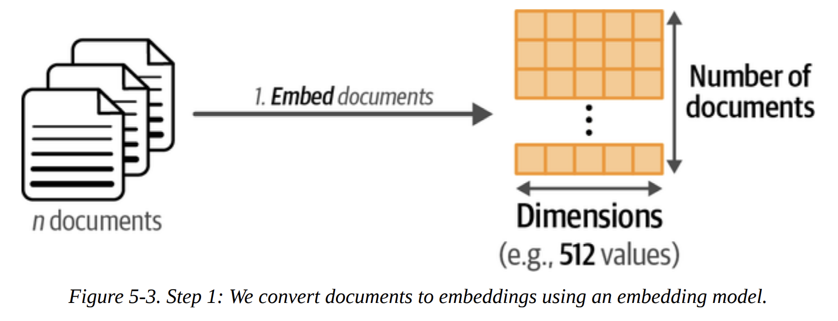
Our first step, shown in Figure 5-3, is to convert the 44,949 abstracts into 44,949 embedding vectors. What are we trying to achieve here? We want vectors where the distance between them reflects semantic similarity. Abstracts about “machine translation” should be close to each other in this vector space, and far from abstracts about “phonetics.”

Choosing the right embedding model is key. The book wisely points to the MTEB (Massive Text Embedding Benchmark) leaderboard. For this task, we want a model that performs well on clustering and is reasonably fast. The book selects thenlper/gte-small, a great choice that balances performance and size.

from sentence_transformers import SentenceTransformer

# Create an embedding for each abstract
embedding_model = SentenceTransformer("thenlper/gte-small")
embeddings = embedding_model.encode(abstracts, 
                                      show_progress_bar=True)

After running this, let’s check the shape of our result.

# Check the dimensions of the resulting embeddings
embeddings.shape

Output: (44949, 384)

This tells us we have 44,949 vectors, each with 384 dimensions. This is our high-dimensional representation of the dataset.

Reducing the Dimensionality of Embeddings

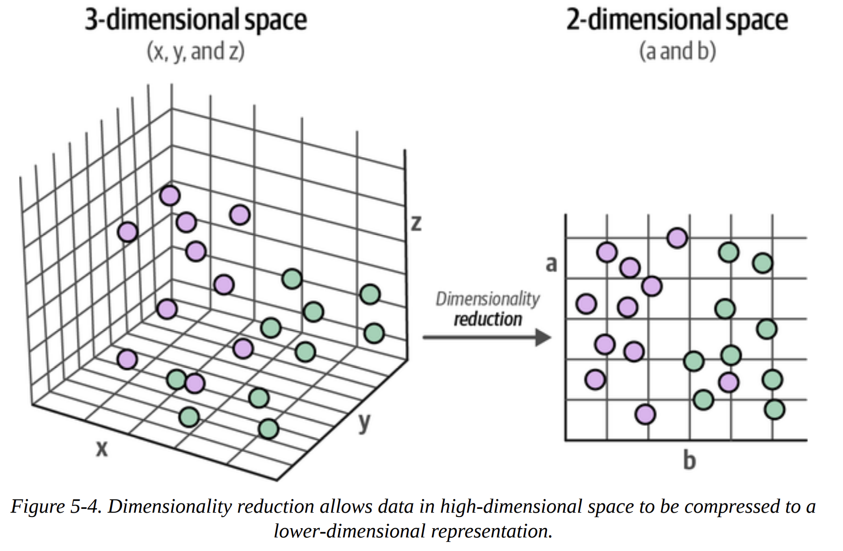
Now, why do we need this step? It comes down to a concept data scientists know well: the curse of dimensionality. In high-dimensional spaces (like 384-D), distances become less meaningful, and everything seems far apart. This makes it very difficult for clustering algorithms to find dense regions.

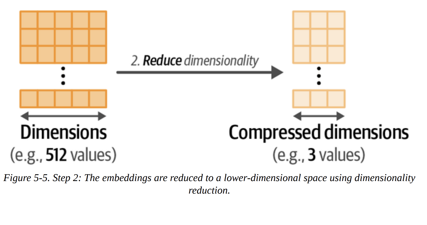
Our goal is to compress this 384-D space into a much lower-dimensional one (e.g., 5-D) while preserving as much of the global structure as possible. We want the points that were close in 384-D to remain close in 5-D. Figure 5-4 and Figure 5-5 visualize this compression perfectly.

The book chooses UMAP (Uniform Manifold Approximation and Projection) over the classic PCA. This is a deliberate choice. UMAP is excellent at preserving the non-linear structures and local/global relationships in the data, which is exactly what we need.

from umap import UMAP

# We reduce the input embeddings from 384 dimensions to 5 dimensions
umap_model = UMAP(n_components=5, 
                  min_dist=0.0, 
                  metric='cosine', 
                  random_state=42)

reduced_embeddings = umap_model.fit_transform(embeddings)

Let’s break down these parameters, as a senior DS would:

• n_components=5: We’re projecting down to 5 dimensions. This is a sweet spot for capturing structure without being too high-dimensional for the clustering algorithm.
• min_dist=0.0: This encourages UMAP to create very tight, dense clusters, which is great for our purpose.
• metric='cosine': We use cosine similarity because it’s generally more effective than Euclidean distance for high-dimensional text embeddings.
• random_state=42: This makes our UMAP results reproducible.

Cluster the Reduced Embeddings

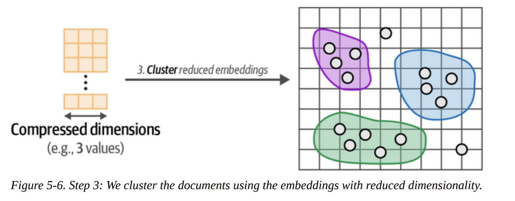
This is the final step in our pipeline, as shown in Figure 5-6. We now have 44,949 points in a 5-D space. Our goal is to assign a cluster label to each point.

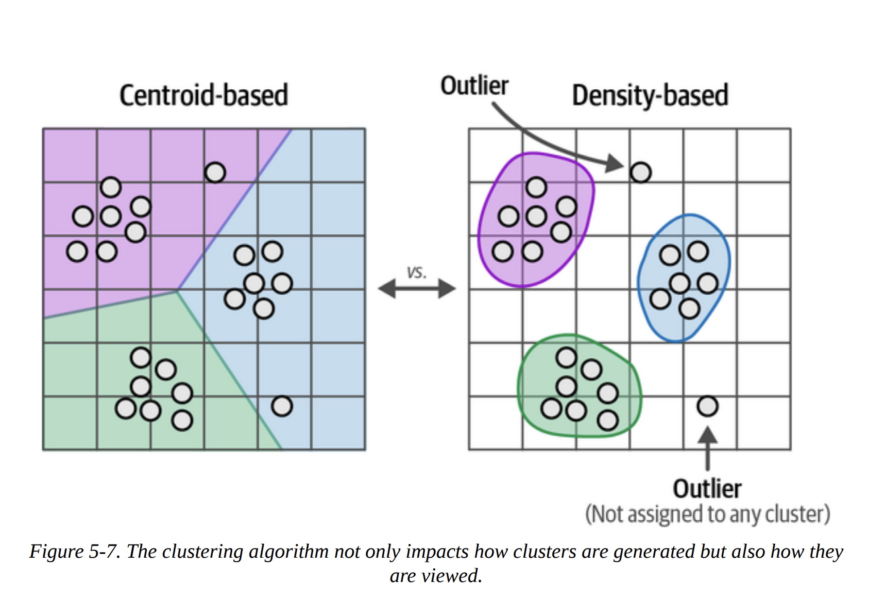
The book makes another excellent point by contrasting centroid-based clustering (like k-means) with density-based clustering (Figure 5-7).

• K-means requires you to specify the number of clusters (k) beforehand. We don’t know k! It also forces every single point into a cluster.
• HDBSCAN (Hierarchical Density-Based Spatial Clustering of Applications with Noise) is a much better fit. It automatically determines the number of clusters based on density and, crucially, it allows for outliers. It identifies points that don’t belong to any dense cluster and labels them as such (typically with -1). Since our ArXiv dataset likely contains many niche or unique papers, this ability to handle outliers is perfect.

from hdbscan import HDBSCAN

# We fit the model and extract the clusters
hdbscan_model = HDBSCAN(min_cluster_size=50, 
                        metric="euclidean", 
                        cluster_selection_method="eom")
                        .fit(reduced_embeddings)

clusters = hdbscan_model.labels_

min_cluster_size=50 tells the algorithm to not even consider a group of points a cluster unless it has at least 50 members. This helps avoid tiny, noisy micro-clusters.

When we check len(set(clusters)), we find we’ve generated 156 clusters.

Inspecting the Clusters

Now we have our clusters, but what do they mean? The book shows how to do a quick manual inspection. Let’s look at the first three documents from Cluster 0.

import numpy as np

# Print first three documents in cluster 0
cluster = 0
for index in np.where(clusters==cluster)[0][:3]:
    print(abstracts[index][:300] + "... \n")

The output shows documents about “statistical machine translation from English text to American Sign Language (ASL)”. It seems Cluster 0 is about Sign Language Translation. This is the core of exploratory analysis!

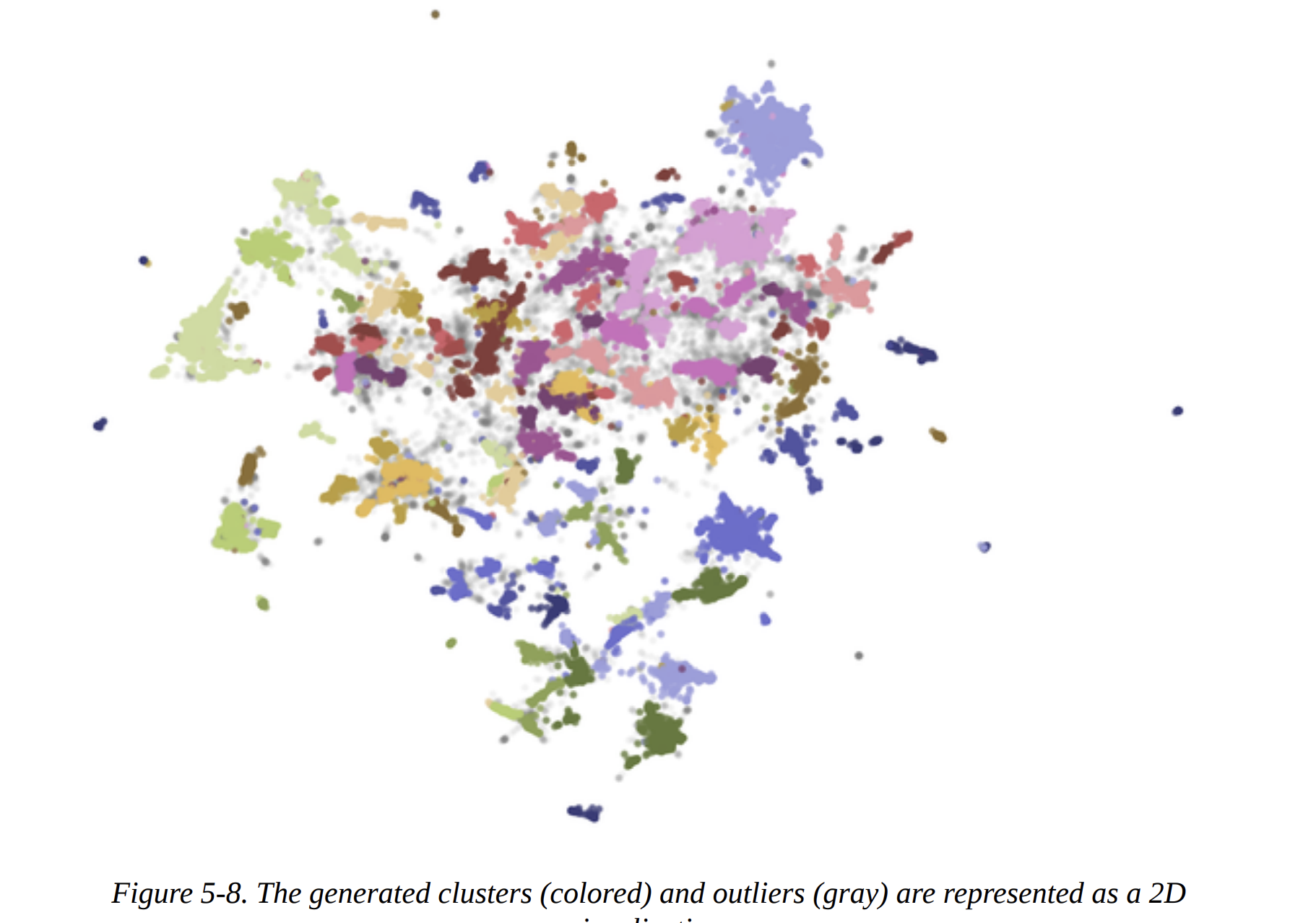
For a bird’s-eye view, we can create the 2D scatter plot shown in Figure 5-8. We re-run UMAP, this time with n_components=2 for visualization, and plot the points, coloring them by their cluster ID. The gray points are the outliers identified by HDBSCAN.

From Text Clustering to Topic Modeling

Manually inspecting clusters is insightful but not scalable. This is where we transition to Topic Modeling. The goal is to automatically generate a representation for each cluster.

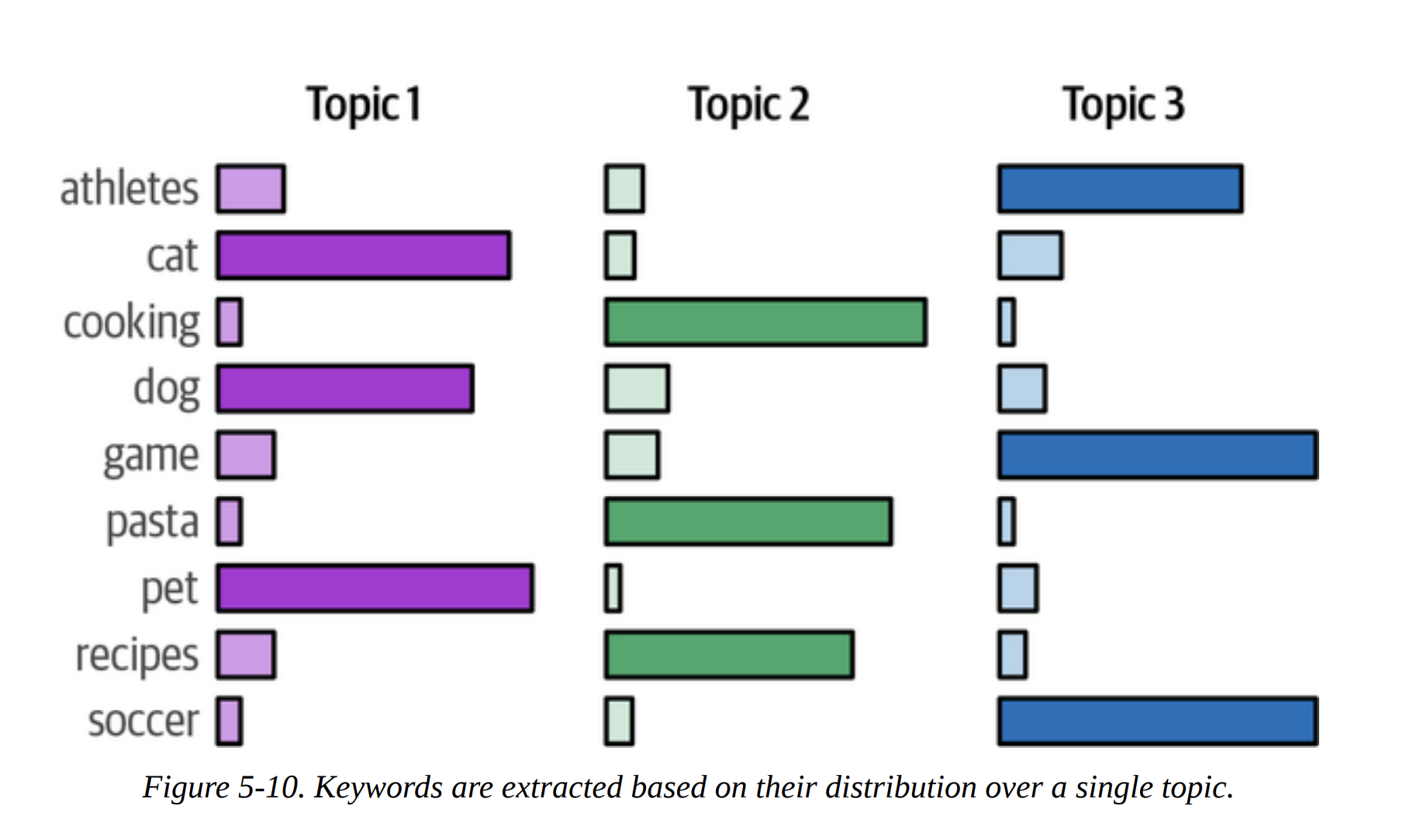
Instead of a single label like “Sign Language,” traditional topic modeling (like Latent Dirichlet Allocation, or LDA) represents a topic as a distribution of words, as shown in Figures 5-9 and 5-10. The top words in the distribution act as the topic’s description.

BERTopic: A Modular Topic Modeling Framework

This is the star of the chapter. BERTopic is a brilliant framework that formalizes and extends the pipeline we just built.

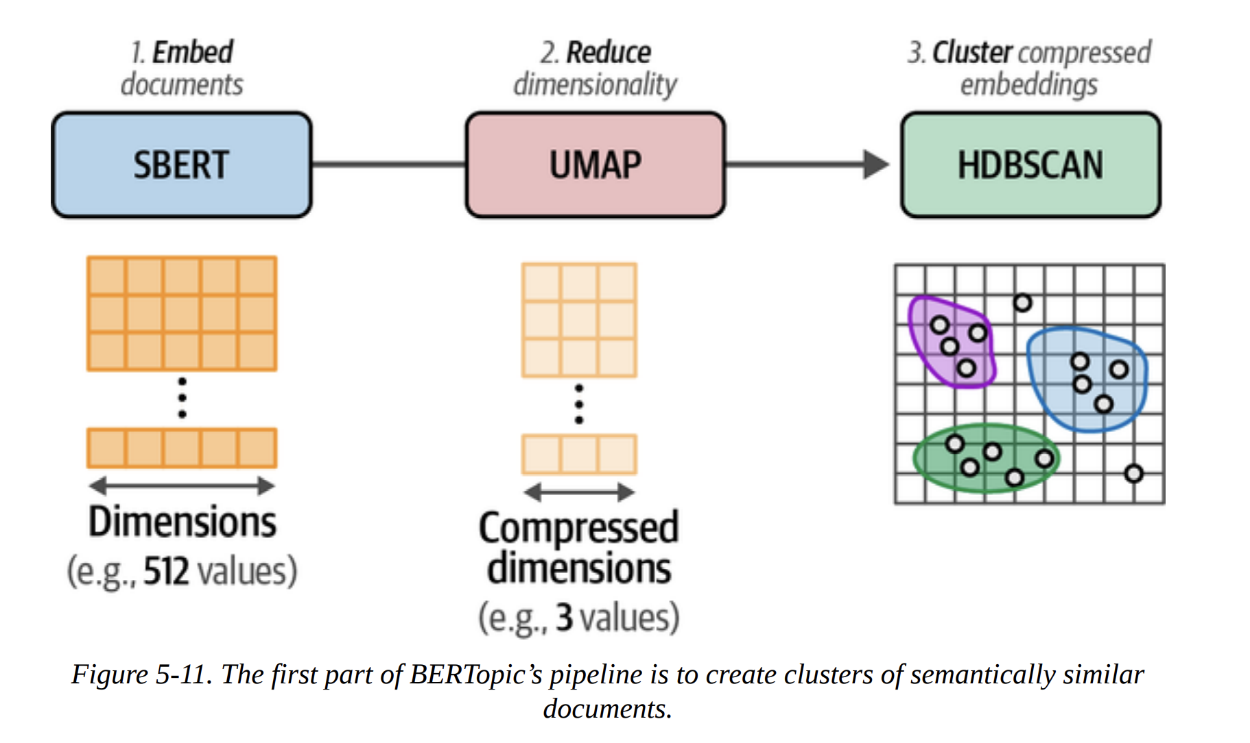
As Figure 5-11 shows, the first part of BERTopic is exactly what we did: SBERT (Embed) -> UMAP (Reduce) -> HDBSCAN (Cluster).

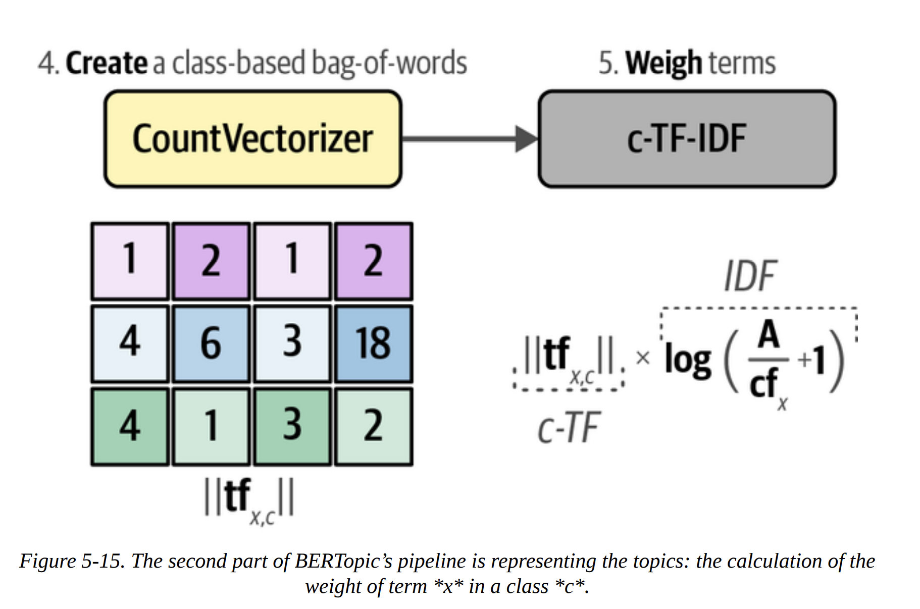
The second part is where it gets clever. How does it represent the topics? It uses a classical NLP technique: c-TF-IDF. Let me break this down, because it’s the secret sauce.

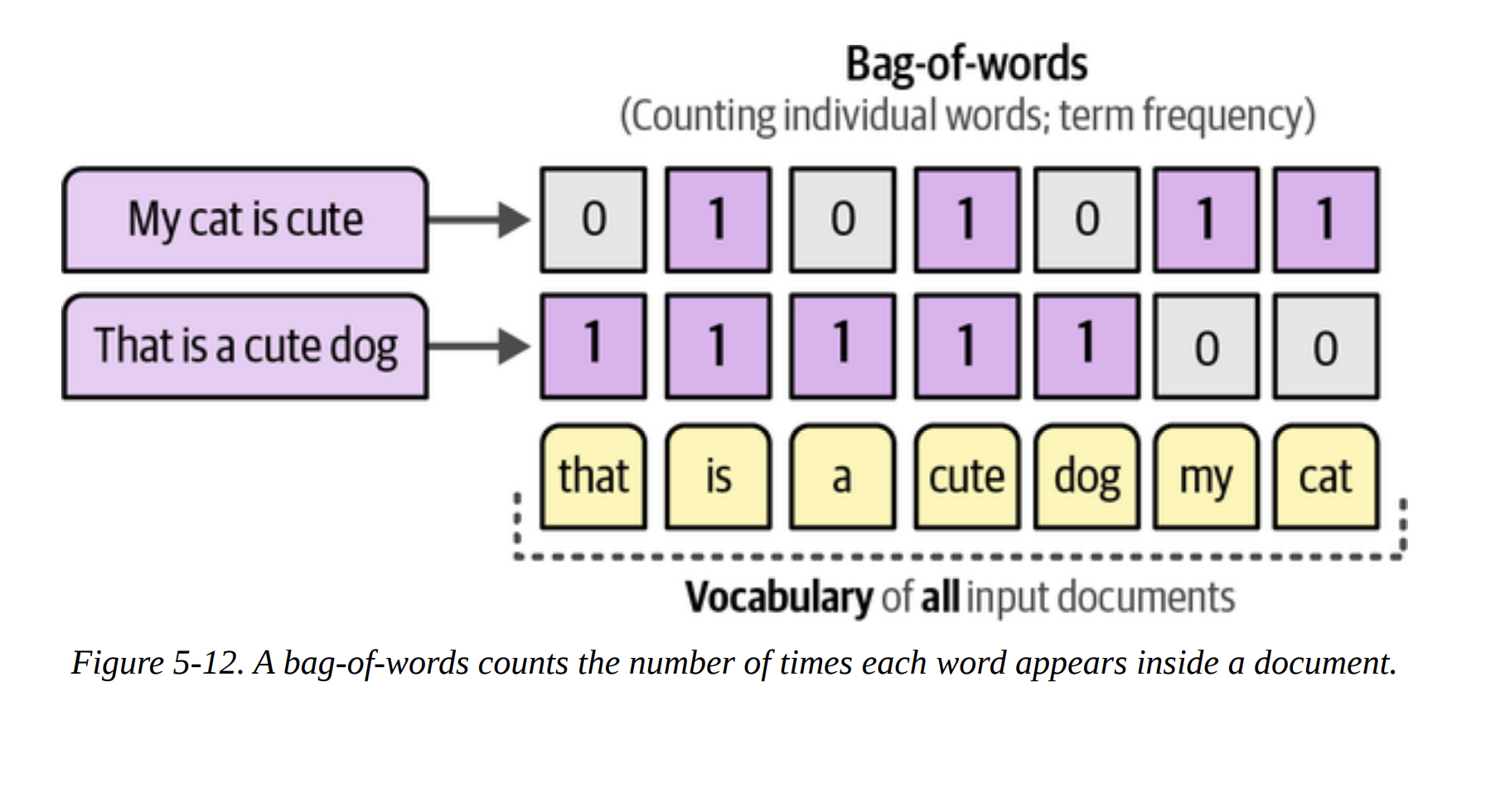
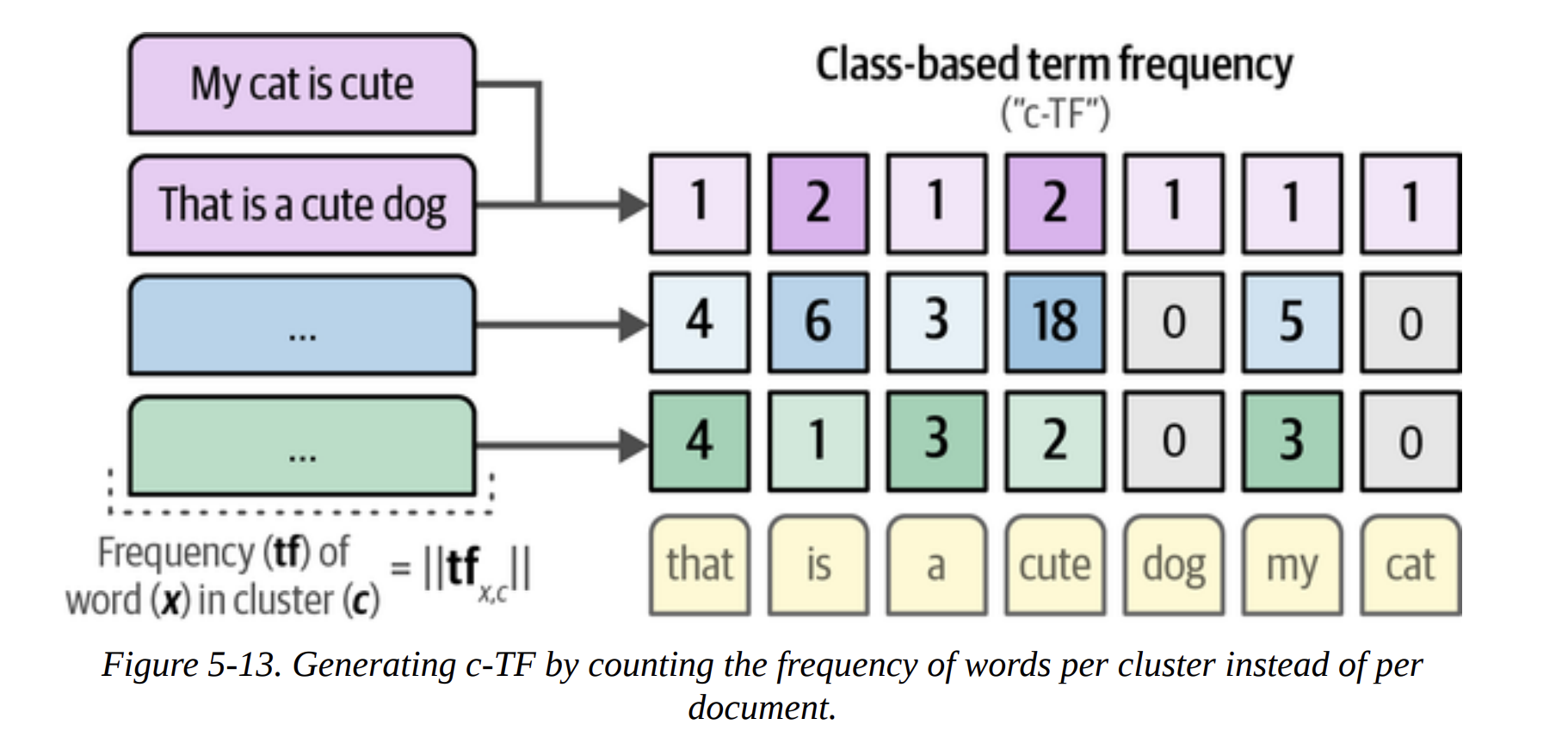
1. Bag-of-Words: First, for all documents within a single cluster, it creates a giant bag-of-words. It’s not per-document, but per-cluster (Figure 5-13). This gives us the Term Frequency (TF) for each word within its class (c). This is the “c-TF” part.

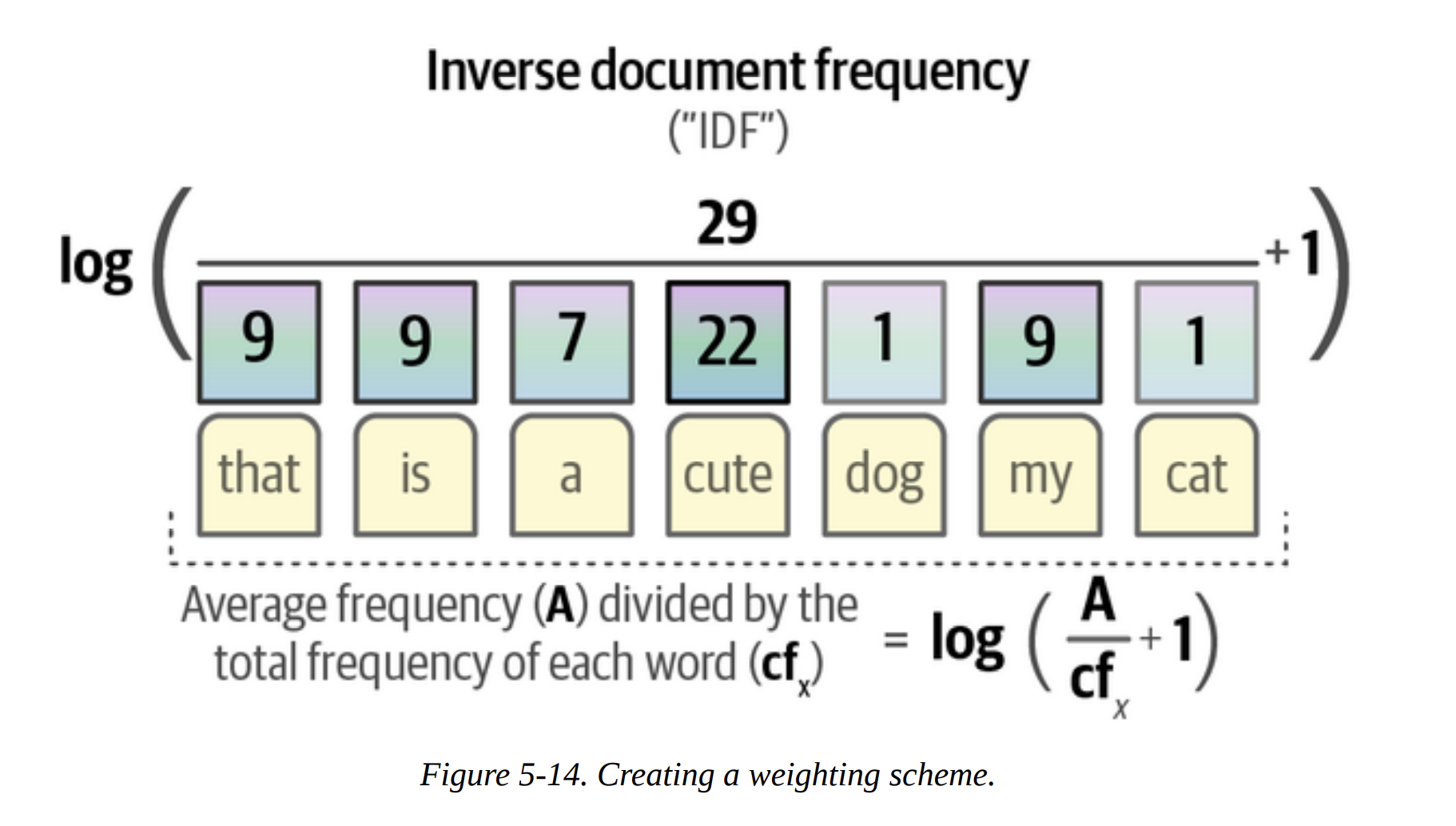
2. Inverse Document Frequency (IDF): It then calculates how common each word is across all clusters. Words that are common everywhere (like the, and, model) are uninformative and get a low IDF score. Words that are frequent in one cluster but rare elsewhere (like asr or phonetic) are very informative and get a high IDF score (Figure 5-14).

3. c-TF-IDF Score: The final score for a word in a topic is c-TF * IDF. This score is high for words that are frequent within a topic but rare overall. These are the perfect keywords to describe the topic!

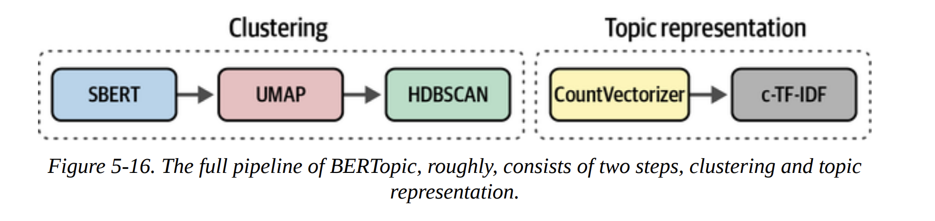
The full BERTopic pipeline is shown in Figure 5-16. It’s this beautiful marriage of modern deep learning for semantic clustering and classic, interpretable TF-IDF for topic representation.

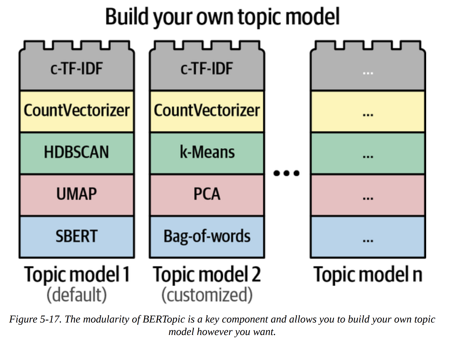
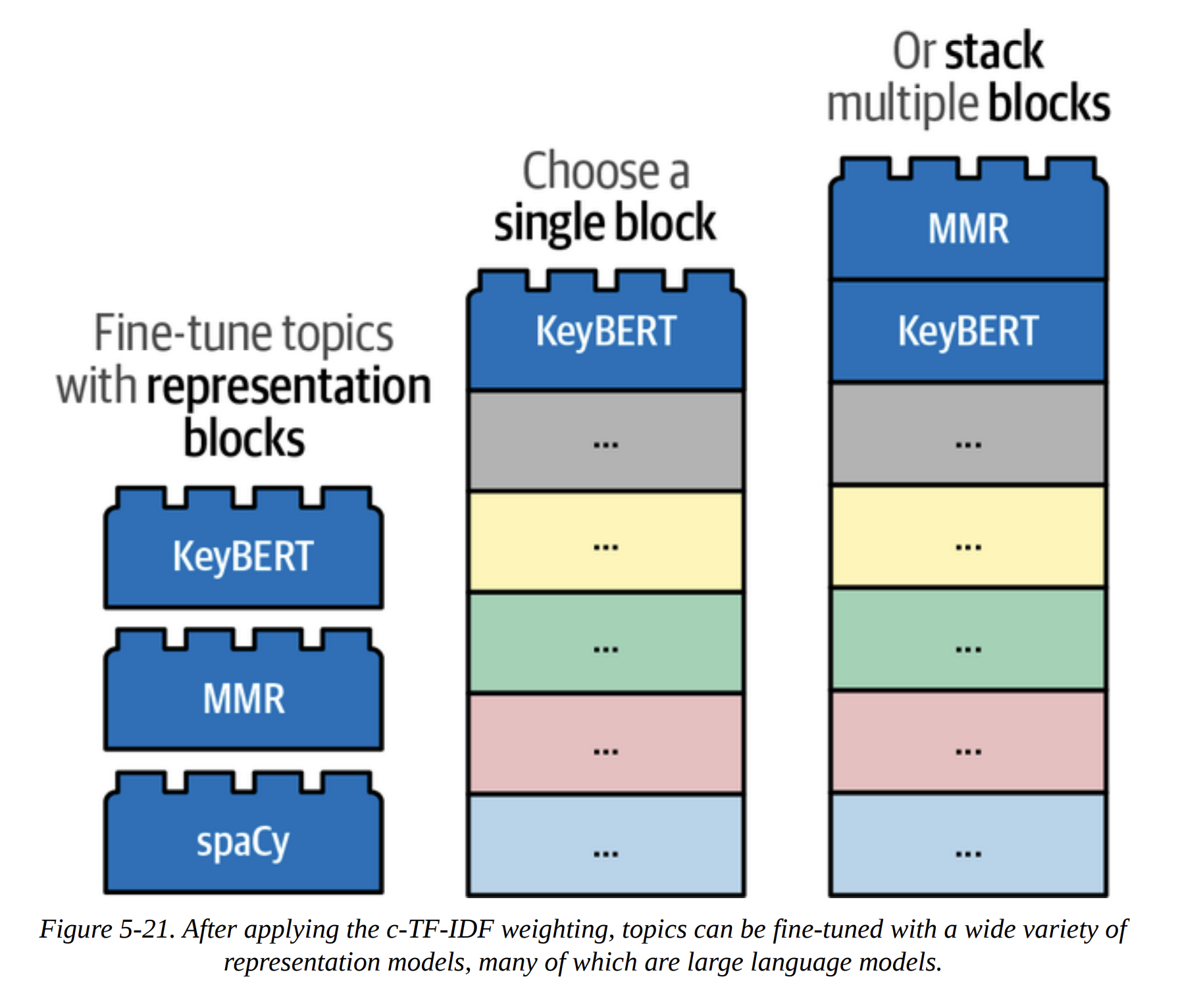
The true power of BERTopic, as emphasized in Figure 5-17, is its modularity. It’s built like Lego blocks. Don’t like HDBSCAN? Swap it for k-means. Have a better embedding model? Plug it in. This makes the framework incredibly powerful and future-proof.

Let’s run it. We can even reuse the components we already trained.

from bertopic import BERTopic

# Train our model with our previously defined models
topic_model = BERTopic(
    embedding_model=embedding_model,
    umap_model=umap_model,
    hdbscan_model=hdbscan_model,
    verbose=True
).fit(abstracts, embeddings)

We can now inspect the topics programmatically.

# Get a summary of the topics
topic_model.get_topic_info()

This gives us a table with the topic ID, the number of documents (Count), and a default Name made from the top 4 keywords. We can see Topic -1 (the outliers), Topic 0 (speech_asr_recognition_end), Topic 1 (medical_clinical_biomedical_pa), and so on.

Adding a Special Lego Block: Representation Models

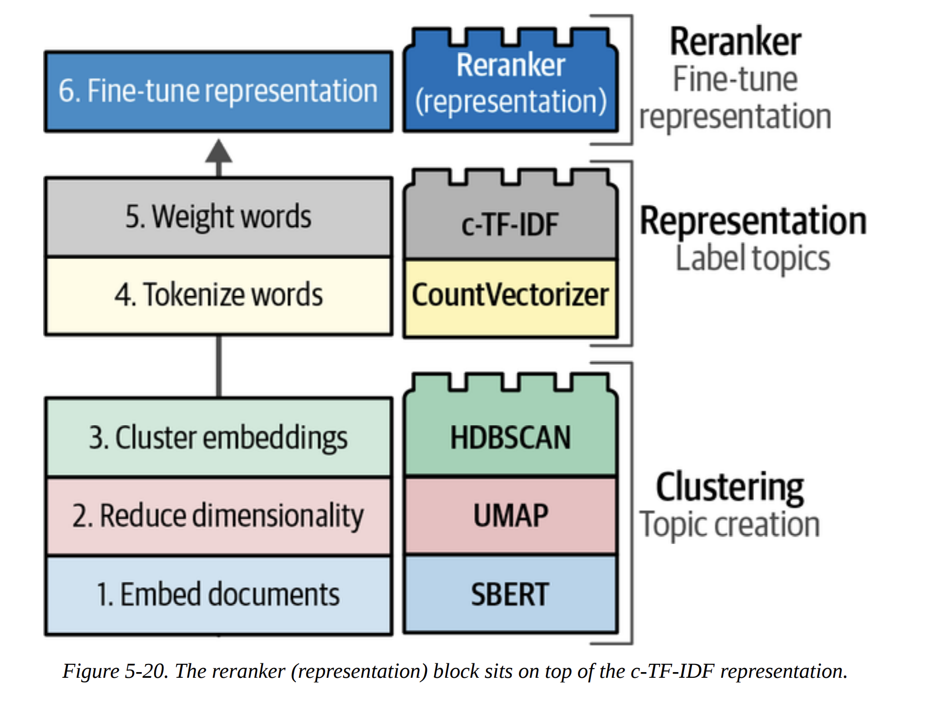
The default c-TF-IDF representation is great, but we can do even better. BERTopic allows us to add new “Lego blocks” on top of the pipeline to rerank or relabel the topics. This is the concept of a Representation Model (Figure 5-20).

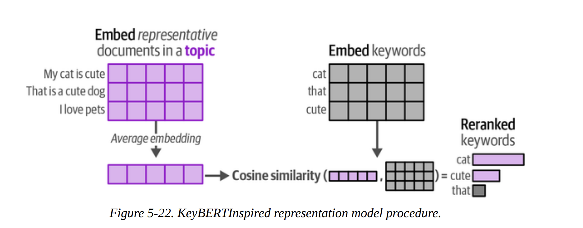
KeyBERTInspired

This method improves the keyword-based representation. What’s the goal? To find keywords that are not just frequent, but are also semantically very similar to the overall meaning of the topic. As shown in Figure 5-22, it calculates the average embedding of all documents in a topic. Then, it finds candidate keywords (from c-TF-IDF) whose own embeddings are most similar to this average topic embedding. This cleans up the keyword list beautifully. The comparison table on page 34 shows the “Original” vs “Updated” keywords, and the updated ones are much more coherent.

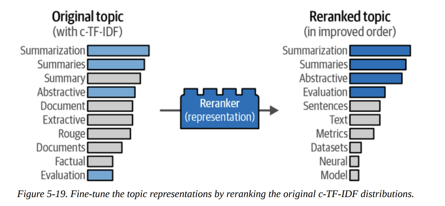
Maximal Marginal Relevance (MMR)

What’s the goal here? To improve diversity. A topic might have keywords like summaries, summary, summarization. They are redundant. MMR is an algorithm that selects a list of keywords that are both relevant to the topic and diverse from each other. The table on page 36 clearly shows this—the updated topic for “summarization” is much more diverse and informative.

The Text Generation Lego Block

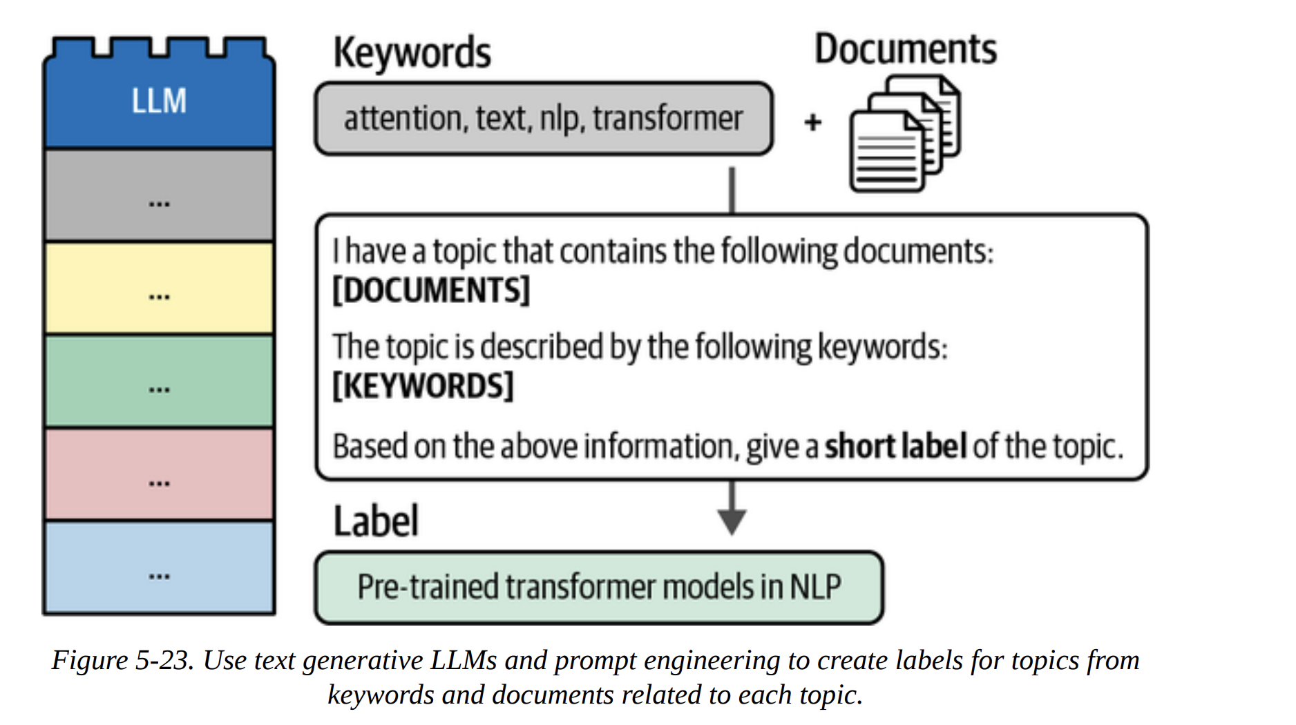
This is the ultimate upgrade. Why just have a list of keywords when we can have a full, human-readable label? Our goal: use a generative LLM to create a short, descriptive title for each topic.

This is incredibly efficient. Instead of running the LLM on millions of documents, we run it just once per topic (156 times in our case). As Figure 5-23 shows, we construct a prompt for the LLM that includes the top keywords and a few representative documents from the topic, and then we ask it: “Based on this, what’s a short label for this topic?”

The book shows examples with both Flan-T5 and GPT-3.5. The results with GPT-3.5 (page 40) are stunningly good:

• Topic 0 (speech, asr, recognition) becomes “Leveraging External Data for Improving Low-Res…”
• Topic 1 (medical, clinical) becomes “Improved Representation Learning for Biomedica…”
• Topic 3 (translation, nmt) becomes “Neural Machine Translation”

These are not just keywords; they are meaningful, high-quality topic labels.

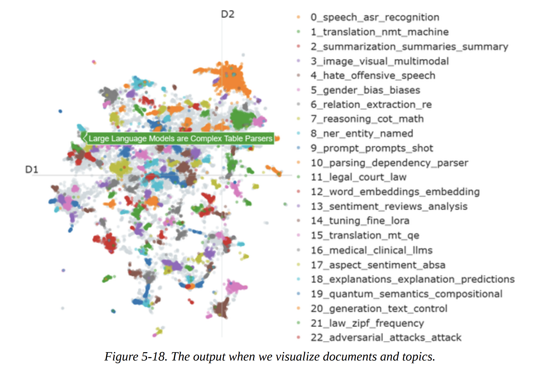
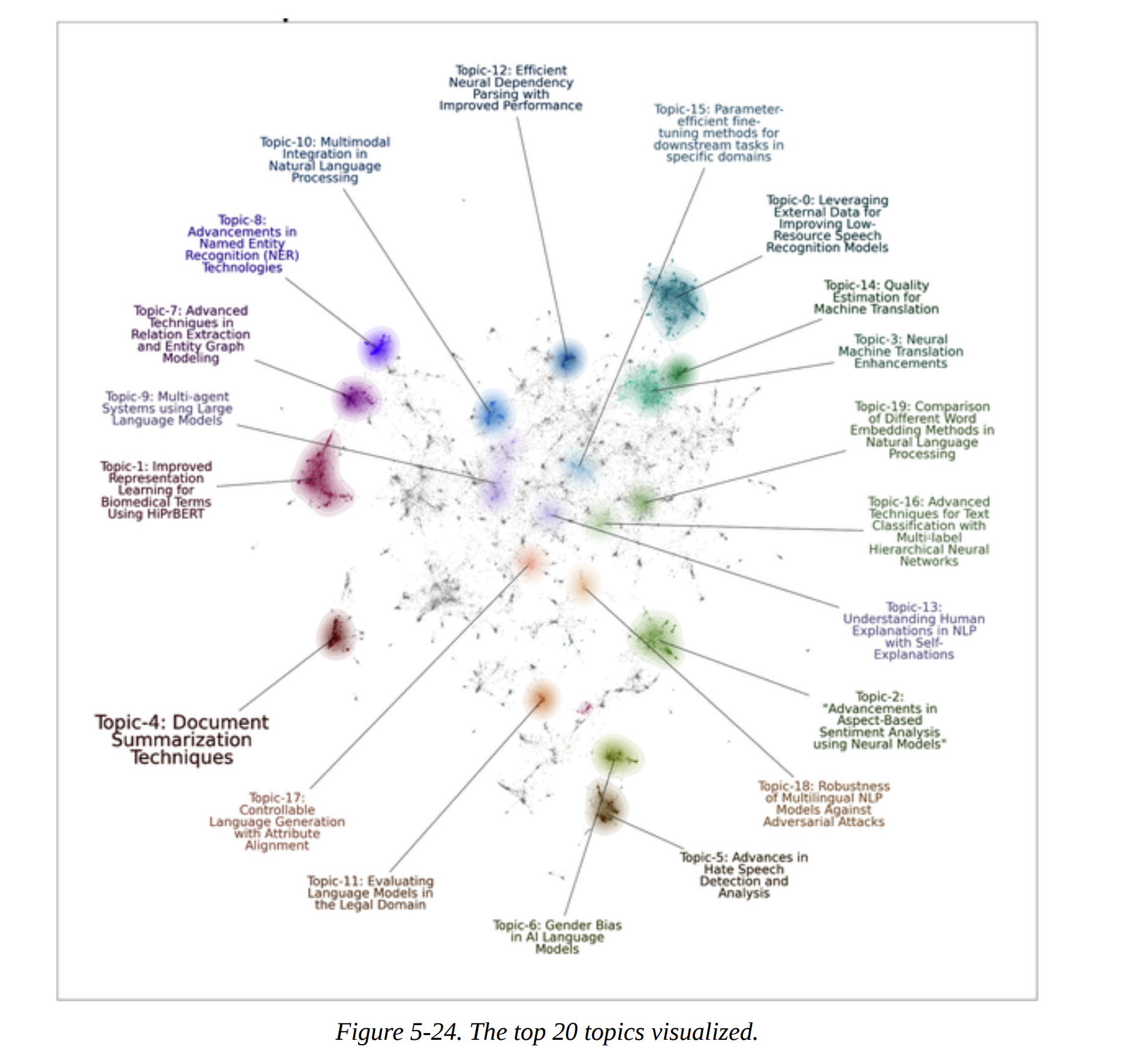
With these amazing labels, we can now create the final, beautiful visualization from Figure 5-24, using the datamapplot package. It plots the documents and adds the generated labels, giving us an interpretable map of the entire dataset.

Summary

And that’s Chapter 5. We’ve gone on a complete journey through unsupervised learning with modern tools.

We started with a foundational three-step clustering pipeline: Embed, Reduce, and Cluster. We made deliberate, expert choices at each step: a strong SentenceTransformer model, UMAP for dimensionality reduction, and HDBSCAN for robust, density-based clustering.

We then saw how BERTopic elegantly packages this pipeline and enhances it with an interpretable c-TF-IDF representation to define topics.

Finally, and most powerfully, we explored the modular “Lego block” nature of BERTopic by adding representation models to refine our topics. We used KeyBERTInspired and MMR to improve keyword quality and diversity, and we capped it all off by using a powerful generative LLM to create high-quality, human-readable labels.