Chapter 10: Introduction to Artificial Neural Networks
39 min readIntroduction - Inspiration from Nature
The chapter beautifully starts by reminding us how nature has often inspired human inventions: birds inspired planes, burdock plants inspired Velcro. So, it’s logical to look at the brain’s architecture for inspiration on building intelligent machines. This is the core idea that sparked ANNs.
ANNs vs. Biological Neurons: While ANNs were inspired by the networks of biological neurons in our brains, they have evolved to be quite different. Just like planes don’t flap their wings, ANNs don’t need to be biologically perfectly realistic to be effective. The footnote mentions a good philosophy: be open to biological inspiration but don’t be afraid to create biologically unrealistic models if they work well. Some researchers even prefer calling the components “units” rather than “neurons” to avoid this restrictive analogy.
The Power of ANNs:
- They are at the heart of Deep Learning.
- Versatile, powerful, and scalable.
- Ideal for large, complex tasks like:
- Image classification (Google Images)
- Speech recognition (Apple’s Siri)
- Recommendation systems (YouTube)
- Game playing (DeepMind’s AlphaGo)
Chapter Structure:
- Part 1: Introduces ANNs, starting from early architectures and leading up to Multilayer Perceptrons (MLPs), which are heavily used today.
- Part 2: Focuses on implementing neural networks using the Keras API. Keras is described as a “beautifully designed and simple high-level API” for building, training, evaluating, and running neural networks.
(Page 280: From Biological to Artificial Neurons - A Brief History)
Early Beginnings (1943): ANNs are surprisingly old! They were first introduced by neurophysiologist Warren McCulloch and mathematician Walter Pitts. Their landmark paper proposed a simplified computational model of how biological neurons might perform complex computations using propositional logic. This was the first ANN architecture.
The First “AI Winter” (1960s-1970s): Early successes led to widespread belief in imminent truly intelligent machines. When this didn’t materialize quickly, funding dried up, and ANNs entered a long “winter.”
Revival (1980s - Connectionism): New architectures and better training techniques sparked renewed interest. However, progress was slow.
The Second “AI Winter” (1990s): Other ML techniques like Support Vector Machines (Chapter 5) emerged, seeming to offer better results and stronger theoretical foundations, pushing ANNs to the background again.
The Current Wave (Now!): We’re in another, much stronger wave of interest in ANNs. Why is this time different?
- Huge Quantity of Data: We now have vast amounts of data to train large neural networks (e.g., ImageNet). ANNs often outperform other ML techniques on very large and complex problems.
- Tremendous Increase in Computing Power:
- Moore’s Law (components in circuits doubling roughly every 2 years).
- Powerful GPUs (Graphics Processing Units), initially driven by the gaming industry, are exceptionally good at the kind of parallel computations needed for ANNs.
- Cloud platforms make this power accessible to everyone.
- Improved Training Algorithms: While often only slight tweaks from 1990s algorithms, these have had a huge positive impact (e.g., better optimization algorithms, initialization techniques, regularization).
- Theoretical Limitations Turning Benign: Fears that ANNs would always get stuck in poor local optima have largely proven less of an issue in practice. When they do get stuck, the local optima are often fairly close to the global optimum.
- Virtuous Circle of Funding and Progress: Amazing products based on ANNs make headlines (AlphaGo, GPT-3/4, etc.), attracting more attention, funding, and talent, leading to further progress.
(Page 281-283: Biological Neurons and a Simple Artificial Neuron Model)
Biological Neurons (Figure 10-1, page 282):
- A quick look at the structure: cell body (soma), dendrites (receive signals), axon (transmits signals), synaptic terminals (connect to other neurons).
- Neurons produce electrical impulses (action potentials). When a neuron receives enough neurotransmitter signals at its synapses within a short period, it “fires” its own impulse. Some neurotransmitters are excitatory (encourage firing), some are inhibitory.
- Individual neurons are relatively simple, but billions of them, each connected to thousands of others, form a vast network capable of highly complex computations. The brain’s architecture, especially the layered structure of the cerebral cortex (Figure 10-2), provides inspiration.
Logical Computations with Artificial Neurons (McCulloch & Pitts Model - Page 283):
- Their early model was very simple:
- Binary (on/off) inputs.
- One binary (on/off) output.
- The neuron activates its output if a certain number of its inputs are active.
- Figure 10-3 shows how such simple neurons can perform basic logical computations (assuming activation if at least two inputs are active):
- Identity (C=A): Neuron A sends two signals to C. If A is on, C gets two active inputs and turns on.
- Logical AND (C = A ∧ B): C activates only if both A and B are active (one active input isn’t enough).
- Logical OR (C = A ∨ B): C activates if A is active, or B is active, or both (any one provides two inputs to a common intermediate neuron, which then activates C, or if A and B both directly input to C and one active input is enough, though the diagram is a bit more complex). The diagram shows intermediate neurons. The idea is that if A is active, it can trigger enough input for C to fire, same for B.
- Complex Logic (e.g., A AND NOT B): If we assume an input can inhibit activity, this is also possible. If A is active and B is off, C activates. If B is on, it inhibits C.
- What this was ultimately trying to achieve: To show that even a very simplified model of a neuron, when networked, could perform fundamental logical computations, suggesting a path towards building computational intelligence.
- Their early model was very simple:
(Page 284-288: The Perceptron)
Invented by Frank Rosenblatt in 1957. One of the simplest ANN architectures.
Based on a Threshold Logic Unit (TLU) or Linear Threshold Unit (LTU) (Figure 10-4, page 284):
- Inputs & Output: Numbers (not just binary on/off).
- Weights: Each input connection
ihas an associated weightwᵢ. - Weighted Sum: The TLU computes a weighted sum of its inputs:
z = w₁x₁ + w₂x₂ + ... + wₙxₙ = wᵀx. - Step Function: It then applies a step function to this sum
zto produce the output:h_w(x) = step(z). - What the TLU is ultimately trying to achieve: It makes a decision based on whether a weighted combination of evidence (
z) exceeds some threshold.
Common Step Functions (Equation 10-1, page 285):
- Heaviside step function: Outputs 0 if
z < 0, outputs 1 ifz ≥ 0(assuming threshold is 0). - Sign function: Outputs -1 if
z < 0, 0 ifz = 0, +1 ifz > 0.
- Heaviside step function: Outputs 0 if
Single TLU for Classification:
- A single TLU can perform simple linear binary classification. It’s very similar to a Logistic Regression or linear SVM classifier, but with a hard threshold output instead of a probability or a margin.
- Example: Classify Iris flowers based on petal length and width. You’d add a bias feature
x₀=1. Training means finding weightsw₀, w₁, w₂.
Perceptron Architecture (Figure 10-5, page 286):
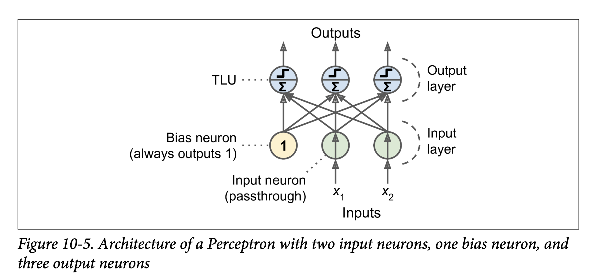
- A Perceptron is typically a single layer of TLUs.
- Each TLU in this layer is connected to all inputs. This is a fully connected layer (or dense layer).
- Inputs are fed through special “passthrough” input neurons.
- A bias neuron (always outputting 1) is usually added and connected to each TLU, providing the bias term
w₀(orbin the new notation used later). - The Perceptron in Figure 10-5 has 2 inputs, 1 bias neuron, and 3 output TLUs. This can classify instances into three different binary classes simultaneously (making it a multioutput classifier). For example, output 1 could be “is it a cat?”, output 2 “is it a dog?”, output 3 “is it a bird?”. An input could be classified as a cat AND a bird if both TLUs fire (though that specific example isn’t ideal for mutually exclusive animal classes).
Computing Outputs for a Layer (Equation 10-2, page 286): For a whole layer of artificial neurons, for several instances at once:
h_W,b(X) = φ(XW + b)X: Matrix of input features (instances x features).W: Weight matrix (input neurons x artificial neurons in the layer). Contains connection weights excluding bias.b: Bias vector (one bias term per artificial neuron in the layer).XW + b: Computes the weighted sumzfor every neuron and every instance.φ(phi): The activation function. For TLUs, this is a step function.- What this equation is ultimately trying to achieve: Efficiently calculate the output of every neuron in a layer for every instance in a batch of data, using matrix multiplication.
Perceptron Training (Hebbian Learning & Perceptron Learning Rule - Page 286):
- Inspired by Hebb’s Rule (“Cells that fire together, wire together”): When neuron A often triggers neuron B, the connection between them strengthens.
- Perceptrons use a variant: The Perceptron learning rule reinforces connections that help reduce the error.
- Process:
- Feed one training instance at a time.
- For each instance, make predictions.
- For every output neuron that produced a wrong prediction, reinforce the connection weights from the inputs that would have contributed to the correct prediction.
- Equation 10-3 (Weight Update Rule):
wᵢⱼ⁽ⁿᵉˣᵗ ˢᵗᵉᵖ⁾ = wᵢⱼ + η(yⱼ - ŷⱼ)xᵢwᵢⱼ: Weight between i-th input and j-th output neuron.η(eta): Learning rate.yⱼ: Target output for j-th neuron.ŷⱼ: Predicted output for j-th neuron.xᵢ: Value of i-th input for the current instance.- What this rule is ultimately trying to achieve:
- If
ŷⱼis correct (yⱼ - ŷⱼ = 0), weights don’t change. - If
ŷⱼis wrong:- If
yⱼ=1andŷⱼ=0(neuron should have fired but didn’t):yⱼ - ŷⱼ = 1. Weightswᵢⱼare increased ifxᵢwas positive (strengthening connections that should have contributed to firing). - If
yⱼ=0andŷⱼ=1(neuron fired but shouldn’t have):yⱼ - ŷⱼ = -1. Weightswᵢⱼare decreased ifxᵢwas positive (weakening connections that wrongly contributed to firing).
- If
- If
Perceptron Convergence Theorem (Page 287): If training instances are linearly separable, Rosenblatt showed this algorithm would converge to a solution (a set of weights that separates the classes).
Scikit-Learn
Perceptronclass: Implements a single-TLU network.from sklearn.linear_model import Perceptronper_clf = Perceptron()per_clf.fit(X, y)- The book notes this is equivalent to
SGDClassifier(loss="perceptron", learning_rate="constant", eta0=1, penalty=None). - Unlike Logistic Regression, Perceptrons output hard predictions (0 or 1), not probabilities. This is one reason to prefer Logistic Regression.
- The book notes this is equivalent to
Limitations of Perceptrons (Minsky & Papert, 1969 - Page 288):
- Highlighted serious weaknesses, famously that Perceptrons (being linear classifiers) cannot solve some trivial problems like the Exclusive OR (XOR) problem (Figure 10-6, left). XOR is not linearly separable.
- This disappointment led to another decline in ANN research (part of the first AI winter).
(Page 288-293: The Multilayer Perceptron (MLP) and Backpropagation)
Overcoming Perceptron Limitations: Stacking Perceptrons (Page 288):
- Limitations can be overcome by stacking multiple layers of Perceptrons. The resulting ANN is a Multilayer Perceptron (MLP).
- Figure 10-6 (right) shows an MLP that can solve the XOR problem. It uses an intermediate “hidden” layer of neurons.
- What the MLP is ultimately trying to achieve: By having hidden layers, MLPs can learn more complex, non-linear decision boundaries. The hidden layers can transform the input features into a new representation where the problem becomes linearly separable for the output layer.
MLP Architecture (Figure 10-7, page 289):
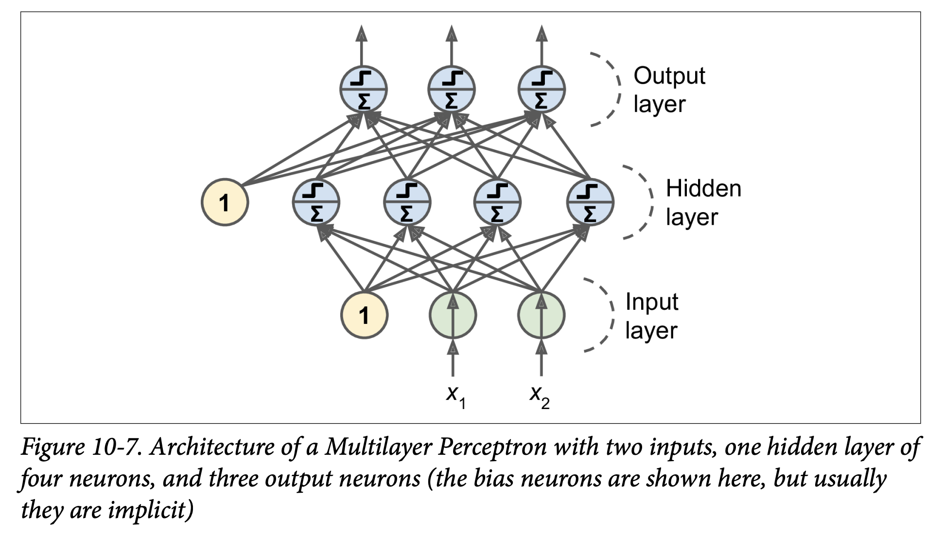
- One (passthrough) input layer.
- One or more layers of TLUs, called hidden layers.
- One final layer of TLUs called the output layer.
- Layers near input are “lower layers”; layers near output are “upper layers.”
- Every layer (except output) usually includes a bias neuron and is fully connected to the next layer.
- Signal flows one way (input -> output): Feedforward Neural Network (FNN).
- Deep Neural Network (DNN): An ANN with a “deep” stack of hidden layers (definition of “deep” is fuzzy but generally means more than one or two these days). Deep Learning studies DNNs.
Training MLPs: The Backpropagation Algorithm (Page 289-290): For many years, training MLPs was a major challenge. In 1986, Rumelhart, Hinton, and Williams published the backpropagation training algorithm, still fundamental today.
- What it is: Essentially, it’s Gradient Descent (Chapter 4) applied to an MLP, using an efficient technique to compute all the necessary gradients.
- How it computes gradients (Autodiff - sidebar, page 290):
- It uses reverse-mode automatic differentiation (autodiff).
- In just two passes through the network (one forward, one backward), it can compute the gradient of the network’s error with respect to every single model parameter (all weights and biases in all layers).
- This tells us how each weight/bias should be tweaked to reduce the error.
- Once gradients are computed, it performs a regular Gradient Descent step. Repeat until convergence.
Backpropagation Algorithm in More Detail (Page 290):
- Mini-batch Processing: Handles one mini-batch of training instances at a time. Goes through the full training set multiple times; each full pass is an epoch.
- Forward Pass:
- Pass the mini-batch to the input layer.
- Compute outputs of neurons in the first hidden layer.
- Pass these outputs to the next layer, compute its outputs, and so on, until the output layer.
- This is like making predictions, but all intermediate results (activations of all neurons) are preserved because they are needed for the backward pass.
- Measure Error: Use a loss function (e.g., MSE for regression, Cross-Entropy for classification) to compare the network’s output with the desired output (true labels).
- Backward Pass (Propagating Error Gradients):
- Compute how much each output connection contributed to the error (using the chain rule of calculus).
- Propagate these error contributions backward:
- Measure how much connections in the layer below contributed to the output layer’s error contributions (again, using chain rule).
- Continue backward until the input layer is reached.
- This reverse pass efficiently measures the error gradient across all connection weights.
- Gradient Descent Step: Tweak all connection weights in the network using the computed error gradients to reduce the overall error.
Key Change for Backpropagation: Activation Functions (Page 291):
- The original Perceptron used a step function. Step functions have flat segments (zero gradient), so Gradient Descent gets stuck.
- Crucial innovation for MLPs: Replace the step function with a differentiable activation function, like the logistic (sigmoid) function
σ(z) = 1 / (1 + exp(-z)).- It has a well-defined, non-zero derivative everywhere, allowing GD to make progress.
- Other Popular Activation Functions (Figure 10-8, page 292):
- Hyperbolic Tangent (tanh):
tanh(z) = 2σ(2z) - 1.- S-shaped, continuous, differentiable.
- Output range: -1 to 1 (vs. 0 to 1 for sigmoid).
- Centering output around 0 often helps speed up convergence at start of training.
- Rectified Linear Unit (ReLU):
ReLU(z) = max(0, z).- Outputs 0 if
z < 0, outputszifz ≥ 0. - Continuous, but not differentiable at
z=0(slope changes abruptly). In practice, GD still works (can use a subgradient or just assume gradient is 0 or 1 atz=0). - Derivative is 0 for
z < 0. - Advantages: Fast to compute. Has become the default in many cases. No maximum output value (helps with some GD issues like vanishing gradients, Ch 11).
- The footnote on page 292 notes that ReLU, despite being less biologically plausible than sigmoids, often works better in ANNs – a case where the biological analogy can be misleading.
- Outputs 0 if
- Hyperbolic Tangent (tanh):
Why Activation Functions? (Page 292):
- If you chain several linear transformations, all you get is another linear transformation.
f(x) = 2x + 3,g(x) = 5x - 1=>f(g(x)) = 2(5x - 1) + 3 = 10x + 1(still linear). - If you have no nonlinearity between layers, even a deep stack of layers is equivalent to a single linear layer. It can’t solve complex non-linear problems.
- Nonlinear activation functions are essential for giving ANNs the power to approximate complex, non-linear functions. A large enough DNN with nonlinear activations can theoretically approximate any continuous function.
- If you chain several linear transformations, all you get is another linear transformation.
(Page 292-294: Regression and Classification MLPs)
Now that we know the architecture and training algorithm (backpropagation), what can we do?
Regression MLPs (Page 292-293):
- Single value prediction (e.g., house price): Need a single output neuron.
- Multivariate regression (e.g., 2D coordinates for object center): One output neuron per output dimension. (4 output neurons if predicting bounding box: x, y, width, height).
- Output Layer Activation:
- Usually no activation function for output neurons in regression (so they can output any range of values).
- If output must be positive: Use ReLU or softplus (
log(1 + exp(z)), a smooth ReLU variant). - If output must be in a specific range: Use logistic (for 0-1) or tanh (for -1 to 1) and scale labels accordingly.
- Loss Function:
- Typically MSE.
- If many outliers: Prefer MAE or Huber loss (quadratic for small errors, linear for large errors – less sensitive to outliers than MSE but converges faster than MAE).
- Table 10-1 (Typical Regression MLP Architecture): Summarizes typical choices for number of neurons, layers, activations, and loss.
Classification MLPs (Page 294):
- Binary classification: Single output neuron, logistic (sigmoid) activation function. Output is probability of positive class.
- Multilabel binary classification (e.g., email is spam/ham AND urgent/non-urgent):
- One output neuron per positive class label (e.g., one for “is spam,” one for “is urgent”).
- Each uses logistic activation.
- Output probabilities don’t necessarily sum to 1 (an email can be “not spam” and “urgent”).
- Multiclass classification (mutually exclusive classes, e.g., digits 0-9):
- One output neuron per class.
- Use softmax activation function for the whole output layer (as in Chapter 4). This ensures probabilities are between 0-1 and sum to 1.
- Figure 10-9 shows a modern MLP for classification (ReLU in hidden layers, softmax in output).
- Loss Function:
- Cross-entropy loss (log loss, as in Chapter 4) is generally a good choice when predicting probability distributions.
- Table 10-2 (Typical Classification MLP Architecture): Summarizes typical choices.
Phew! That’s a dense introduction to the historical context, the biological inspiration (and divergence from it), the basic Perceptron, the jump to Multilayer Perceptrons, the crucial backpropagation algorithm, and how MLPs are structured for regression and classification.
The key takeaway is that MLPs are layered networks of simple processing units (neurons), where hidden layers learn increasingly complex representations of the input, enabled by non-linear activation functions and trained by backpropagation (Gradient Descent with efficient gradient calculation).
Excellent! That detour through “The Matrix Calculus You Need For Deep Learning” was intense but hopefully gave you a much deeper appreciation for what’s happening when we say a neural network “learns” by minimizing a loss function using gradients. You now have a good intuitive (and even some mathematical) backing for how those weight and bias updates are calculated for individual neurons via the chain rule.
(Page 295-306: Implementing MLPs with Keras)
This is where the practical fun begins! We’ve talked a lot about the “what” and “why” of neural networks; now we get to the “how” of actually building and training them using a popular library.
Keras: A High-Level Deep Learning API (Page 295):
- Keras allows you to easily build, train, evaluate, and run all sorts of neural networks.
- It was developed by François Chollet and is known for its ease of use, flexibility, and beautiful design.
- Backend Reliance: Keras itself doesn’t do the heavy numerical computations. It relies on a computation backend. Popular choices include:
- TensorFlow
- Microsoft Cognitive Toolkit (CNTK)
- Theano (though its development has largely ceased)
- The book refers to the original, multi-backend implementation as multibackend Keras.
- tf.keras: Since late 2016/2017, TensorFlow has bundled its own Keras implementation called
tf.keras. This is what the book (and most of the community now) uses. It only supports TensorFlow as a backend but offers extra TensorFlow-specific features (like the Data API for efficient data loading, which we’ll see later). - Figure 10-10 (page 296) illustrates these two Keras API implementations.
PyTorch (Page 296):
- Another very popular Deep Learning library from Facebook.
- Its API is quite similar to Keras (both inspired by Scikit-Learn and Chainer).
- Gained immense popularity due to its simplicity and excellent documentation, especially compared to TensorFlow 1.x.
- TensorFlow 2.x (which uses
tf.kerasas its official high-level API) has significantly improved, making it just as simple as PyTorch in many respects. Healthy competition is good!
Installing TensorFlow 2 (Page 296):
- The book assumes you’ve followed Chapter 2’s setup for Jupyter and Scikit-Learn.
- You’d typically use
pip install -U tensorflow. - The bird icon notes that for GPU support, you might need
tensorflow-gpuand extra libraries (though this is evolving, and TensorFlow aims for a single library). Chapter 19 will cover GPUs. - Test installation by importing
tensorflow as tfandfrom tensorflow import keras, then printingtf.__version__andkeras.__version__.
Now, let’s build an image classifier!
Building an Image Classifier Using the Sequential API (Page 297-301)
We’ll use the Fashion MNIST dataset.
A drop-in replacement for MNIST (introduced in Chapter 3).
Same format: 70,000 grayscale images of 28x28 pixels, 10 classes.
Images are fashion items (T-shirt, trouser, coat, etc.) instead of handwritten digits.
More challenging than MNIST (e.g., a simple linear model gets ~92% on MNIST but only ~83% on Fashion MNIST).
Using Keras to Load the Dataset (Page 297):
fashion_mnist = keras.datasets.fashion_mnist(X_train_full, y_train_full), (X_test, y_test) = fashion_mnist.load_data()- Difference from Scikit-Learn’s
fetch_openmlfor MNIST:- Images are 28x28 arrays (not flattened 784-element vectors).
- Pixel intensities are integers (0-255), not floats.
X_train_full.shapeis(60000, 28, 28).
- Difference from Scikit-Learn’s
Data Preparation (Page 298):
- Create a validation set: The loaded data is split into train and test only. We need a validation set for monitoring training and hyperparameter tuning.
X_valid, X_train = X_train_full[:5000], X_train_full[5000:]y_valid, y_train = y_train_full[:5000], y_train_full[5000:](First 5000 instances for validation, rest for training). - Scale input features: Neural networks with Gradient Descent require feature scaling. We’ll scale pixel intensities from 0-255 down to the 0-1 range by dividing by 255.0 (this also converts them to floats).
X_valid, X_train = X_valid / 255.0, X_train / 255.0(Note: It’s generally better to scale the test set using parameters derived from the training set, e.g.,(X_test - X_train_mean) / X_train_std. But for pixel values 0-255, dividing by 255.0 is a common and simple approach.)
- Class Names: For Fashion MNIST, labels are numbers (0-9). We need a list of class names to interpret them:
class_names = ["T-shirt/top", "Trouser", ..., "Ankle boot"]class_names[y_train[0]]might give'Coat'. - Figure 10-11 shows sample images from Fashion MNIST.
- Create a validation set: The loaded data is split into train and test only. We need a validation set for monitoring training and hyperparameter tuning.
Creating the Model Using the Sequential API (Page 299): This is the simplest way to build a Keras model: a linear stack of layers. We’ll build a classification MLP with two hidden layers.
model = keras.models.Sequential()model.add(keras.layers.Flatten(input_shape=[28, 28]))model.add(keras.layers.Dense(300, activation="relu"))model.add(keras.layers.Dense(100, activation="relu"))model.add(keras.layers.Dense(10, activation="softmax"))Let’s break this down:
model = keras.models.Sequential(): Creates a Sequential model, which is just a stack of layers.model.add(keras.layers.Flatten(input_shape=[28, 28])):- This is the first layer. Its role is to take each input image (28x28 array) and flatten it into a 1D array (of 784 pixels).
X.reshape(-1, 1)was mentioned, but a common operation in NNs isX.reshape(batch_size, -1). Keras Flatten layer handles this conversion. - It has no parameters to learn; it’s just a preprocessing step.
input_shape=[28, 28]: Since it’s the first layer, you must specify the shape of the input instances (excluding the batch size).
- This is the first layer. Its role is to take each input image (28x28 array) and flatten it into a 1D array (of 784 pixels).
model.add(keras.layers.Dense(300, activation="relu")):- Adds a Dense (fully connected) hidden layer with 300 neurons.
activation="relu": Specifies the ReLU activation function for these neurons.- Each
Denselayer manages its own weight matrix (W) and bias vector (b). When it receives input, it computesXW + b(Equation 10-2 from the book).
model.add(keras.layers.Dense(100, activation="relu")):- Adds a second Dense hidden layer with 100 neurons, also using ReLU.
model.add(keras.layers.Dense(10, activation="softmax")):- Adds a Dense output layer with 10 neurons (one for each class, 0-9).
activation="softmax": Uses the softmax activation function because the classes are exclusive (an item belongs to only one class). Softmax will ensure the outputs are probabilities that sum to 1.
- Alternative Sequential Model Creation (Page 300):
You can also pass a list of layers directly to the
Sequentialconstructor:model = keras.models.Sequential([keras.layers.Flatten(input_shape=[28, 28]),keras.layers.Dense(300, activation="relu"),keras.layers.Dense(100, activation="relu"),keras.layers.Dense(10, activation="softmax")])
Model Summary (Page 300-301):
model.summary()displays all the model’s layers:- Layer name (auto-generated or custom).
- Output shape (
Nonefor batch size means it can be anything). - Number of parameters.
Flatten: Output shape(None, 784), 0 params.dense(first hidden layer): Output(None, 300). Params:(784 inputs * 300 neurons) + 300 biases = 235,200 + 300 = 235,500.dense_1(second hidden): Output(None, 100). Params:(300 inputs * 100 neurons) + 100 biases = 30,000 + 100 = 30,100.dense_2(output): Output(None, 10). Params:(100 inputs * 10 neurons) + 10 biases = 1,000 + 10 = 1,010.- Total params: 266,610. All are trainable.
- This gives the model a lot of flexibility but also risks overfitting if data is scarce.
Accessing Layers and Weights (Page 301):
model.layersgives a list of layers.hidden1 = model.layers[1]hidden1.namemodel.get_layer('dense')(if name is ‘dense’)weights, biases = hidden1.get_weights()gets the layer’s parameters.- Weights are initialized randomly (to break symmetry for backpropagation).
- Biases are initialized to zeros (which is fine).
- You can set custom initializers for weights (
kernel_initializer) or biases (bias_initializer) when creating the layer. (More in Ch 11).
When
input_shapeis Determined (Bird Icon, page 302): It’s best to specifyinput_shapefor the first layer. If you don’t, Keras waits until it sees actual data (e.g., duringfit()) or until you callmodel.build()to build the layers (i.e., create their weights). Before that, layers won’t have weights, andmodel.summary()or saving the model might not work.
(Page 302-306: Compiling, Training, Evaluating, and Predicting)
Compiling the Model (Page 302): After creating the model, you must call
compile()to specify:- Loss function
- Optimizer
- Optionally, extra metrics to compute during training/evaluation.
model.compile(loss="sparse_categorical_crossentropy",optimizer="sgd",metrics=["accuracy"])loss="sparse_categorical_crossentropy":- We use this because our labels (
y_train) are “sparse” – just target class indices (0 to 9). - And the classes are exclusive.
- If labels were one-hot encoded (e.g., class 3 is
[0,0,0,1,0,0,0,0,0,0]), we’d useloss="categorical_crossentropy". - If binary classification (output layer with sigmoid), we’d use
loss="binary_crossentropy". - The bird icon (page 302) notes you can use full Keras objects too:
loss=keras.losses.sparse_categorical_crossentropy.
- We use this because our labels (
optimizer="sgd":- This means use simple Stochastic Gradient Descent. Keras will perform backpropagation (reverse-mode autodiff + Gradient Descent).
- More advanced optimizers in Chapter 11.
- Important (bird icon, page 303): For SGD, tuning the learning rate is crucial. You’d typically use
optimizer=keras.optimizers.SGD(learning_rate=...)instead of the string"sgd"(which defaults tolr=0.01).
metrics=["accuracy"]:- Since it’s a classifier, we want to track accuracy during training and evaluation.
Training and Evaluating the Model (Page 303-304): Call
fit():history = model.fit(X_train, y_train, epochs=30,validation_data=(X_valid, y_valid))- Pass input features (
X_train) and target classes (y_train). epochs=30: Number of times to iterate over the entire training dataset. (Defaults to 1, which is usually not enough).validation_data=(X_valid, y_valid): Optional. Keras will measure loss and metrics on this validation set at the end of each epoch. Very useful to see how well the model is generalizing and to detect overfitting.- Output during training: For each epoch, Keras displays:
- Progress bar.
- Mean training time per sample.
- Loss and accuracy on the training set (average over the epoch).
- Loss and accuracy on the validation set (at the end of the epoch).
- The example output shows training loss decreasing and validation accuracy reaching ~89% after 30 epochs. Training and validation accuracy are close, so not much overfitting.
- The bird icon (page 304) mentions
validation_split=0.1as an alternative tovalidation_data, to use the last 10% of training data for validation (before shuffling). - Also mentions
class_weight(to give more importance to underrepresented classes) andsample_weight(for per-instance weighting) arguments infit().
- Pass input features (
Learning Curves (Page 304-305):
fit()returns aHistoryobject.history.historyis a dictionary containing the loss and metrics measured at the end of each epoch (e.g.,loss,accuracy,val_loss,val_accuracy).- You can use this to plot learning curves with pandas and Matplotlib (Figure 10-12, page 305).
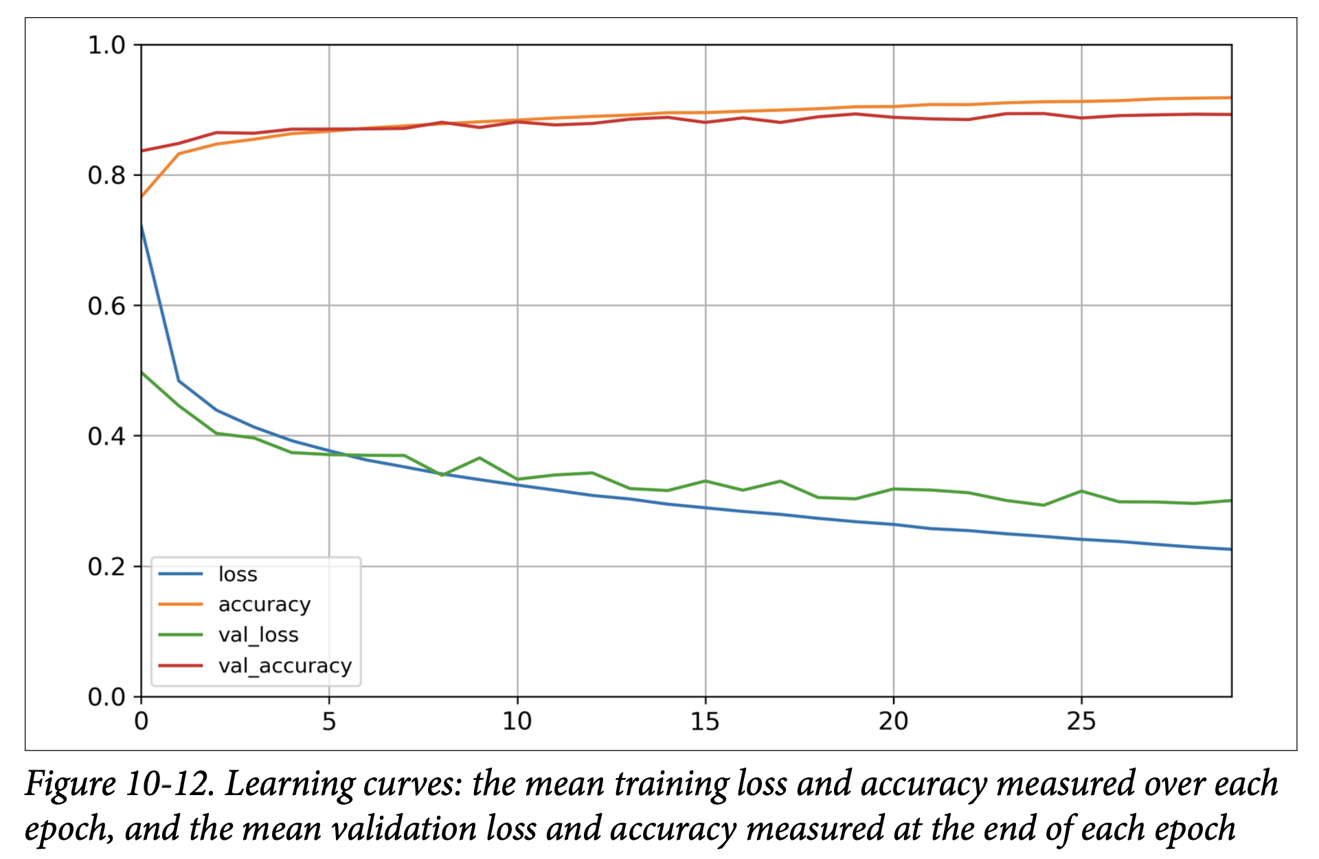
- The plot shows training/validation accuracy increasing and loss decreasing. Validation curves are close to training curves, confirming little overfitting.
- The book notes that validation metrics are computed at the end of an epoch, while training metrics are a running mean during the epoch. So, for a fair comparison, the training curve should be shifted left by half an epoch.
Further Training and Hyperparameter Tuning (Page 306):
- If validation loss is still decreasing (as in the example), the model hasn’t fully converged. You can call
fit()again; Keras continues training from where it left off. - If not satisfied, tune hyperparameters:
- Learning rate (most important first check).
- Try another optimizer (and retune learning rate).
- Number of layers, neurons per layer, activation functions.
- Batch size (in
fit(), defaults to 32).
- If validation loss is still decreasing (as in the example), the model hasn’t fully converged. You can call
Evaluating on the Test Set (Page 306):
- Once satisfied with validation accuracy, evaluate on the test set to estimate generalization error.
model.evaluate(X_test, y_test)Returns[loss, accuracy]. Example gives ~88.5% accuracy. - Common to get slightly lower performance on test set than validation (since HPs tuned on validation). Resist tweaking HPs based on test set results!
- Once satisfied with validation accuracy, evaluate on the test set to estimate generalization error.
Using the Model to Make Predictions (Page 206-207):
predict()method for new instances.X_new = X_test[:3]y_proba = model.predict(X_new)y_probacontains one probability per class for each instance (from the softmax output layer). Example:[[0. , ..., 0.03, ..., 0.96], ...]for the first image (96% prob for class 9 ‘Ankle boot’, 3% for class 5 ‘Sandal’).- To get the class with the highest probability:
y_pred = model.predict_classes(X_new)(Note:predict_classesis deprecated in newer TensorFlow/Keras; usenp.argmax(model.predict(X_new), axis=-1)instead). This might givearray([9, 2, 1]). - Figure 10-13 (page 307) shows these three test images, which were correctly classified.
That’s a complete walkthrough of building, training, and using a classification MLP with Keras’s Sequential API! The process is quite streamlined.
Great! It’s satisfying to see how those theoretical concepts translate into a working Keras model.
Let’s continue with Chapter 10, moving on to how we’d build a regression MLP with Keras and then explore more advanced ways to define model architectures.
(Page 307-308: Building a Regression MLP Using the Sequential API)
We’ve just built an image classifier. Now, let’s switch to a regression task: predicting California housing prices, similar to what we did in Chapter 2, but this time with a neural network.
Loading the Data:
For simplicity, the book uses Scikit-Learn’s
fetch_california_housing()to load the data.This version is simpler than the one in Chapter 2: only numerical features, no missing values.
Standard train-validation-test split and feature scaling (using
StandardScaler) are performed as usual.from sklearn.datasets import fetch_california_housingfrom sklearn.model_selection import train_test_splitfrom sklearn.preprocessing import StandardScalerhousing = fetch_california_housing()X_train_full, X_test, y_train_full, y_test = train_test_split(housing.data, housing.target)X_train, X_valid, y_train, y_valid = train_test_split(X_train_full, y_train_full)scaler = StandardScaler()X_train = scaler.fit_transform(X_train)X_valid = scaler.transform(X_valid)X_test = scaler.transform(X_test)
Building the Regression MLP (Page 308): The process is very similar to the classification MLP, with a few key differences:
model = keras.models.Sequential([keras.layers.Dense(30, activation="relu", input_shape=X_train.shape[1:]),keras.layers.Dense(1) # Output layer])- Output Layer:
- Has a single neuron (because we’re predicting a single value – the housing price).
- Uses no activation function (or you could say a “linear” activation
activation=None). This allows the output neuron to produce any range of values, which is what we want for regression. (Recall for classification we usedsoftmaxorsigmoid).
- Hidden Layer: The example uses a single hidden layer with 30 neurons and ReLU activation. The book mentions using fewer neurons and a shallower network because the dataset is quite noisy, to avoid overfitting.
input_shape=X_train.shape[1:]correctly sets the input dimension based on the number of features inX_train. - What this architecture is ultimately trying to achieve: The hidden layer learns complex combinations of the input features, and the final output neuron combines these learned features linearly to produce the price prediction.
- Output Layer:
Compiling the Model:
model.compile(loss="mean_squared_error", optimizer="sgd")- Loss Function:
loss="mean_squared_error"(orkeras.losses.mean_squared_error). This is standard for regression. - Optimizer:
"sgd"(again, you’d likely want to specifykeras.optimizers.SGD(learning_rate=...)for tuning). - Metrics: For regression, common metrics might be MAE (Mean Absolute Error) if MSE is the loss, or just watching the loss itself. Accuracy isn’t used for regression.
- Loss Function:
Training, Evaluating, Predicting: These steps are identical to the classification MLP:
history = model.fit(X_train, y_train, epochs=20, validation_data=(X_valid, y_valid))mse_test = model.evaluate(X_test, y_test)y_pred = model.predict(X_new)The core workflow with the Sequential API is consistent. The main changes for regression are the structure of the output layer (number of neurons, no activation) and the choice of loss function (MSE).
(Page 308-312: Building Complex Models Using the Functional API)
The Sequential API is easy to use for simple stacks of layers. However, sometimes you need to build neural networks with more complex topologies:
- Multiple inputs.
- Multiple outputs.
- Layers that branch off and then merge back.
For these, Keras offers the Functional API.
Wide & Deep Neural Network (Example Architecture - Page 308, Figure 10-14):
- Introduced in a 2016 paper by Google for recommender systems.
- The Idea: Combine the strengths of deep learning (learning complex patterns through a “deep path” of stacked layers) with the ability to learn simple rules (through a “wide path” where inputs connect directly, or via a shallow path, to the output).
- What it’s ultimately trying to achieve: Prevent simple, easily learnable patterns in the data from being distorted or lost by forcing them through many layers of transformations. It allows the network to memorize simple rules while also discovering intricate patterns.
Building a Wide & Deep Network with the Functional API (Page 309): Let’s tackle the California housing problem with this architecture.
input_ = keras.layers.Input(shape=X_train.shape[1:])hidden1 = keras.layers.Dense(30, activation="relu")(input_)hidden2 = keras.layers.Dense(30, activation="relu")(hidden1)concat = keras.layers.Concatenate()([input_, hidden2])output = keras.layers.Dense(1)(concat)model = keras.Model(inputs=[input_], outputs=[output])Let’s break this down step-by-step:
input_ = keras.layers.Input(shape=X_train.shape[1:]):- This creates an
Inputobject (a symbolic tensor). It defines the shape anddtypeof the input the model will receive. This is like declaring the entry point for your data.
- This creates an
hidden1 = keras.layers.Dense(30, activation="relu")(input_):- We create a
Denselayer. - Then, we call it like a function, passing it the
input_object. This connectsinput_tohidden1.hidden1now represents the symbolic output of this layer. - This “calling a layer on a tensor” is the essence of the Functional API. You are defining how layers connect. No actual data is processed yet.
- We create a
hidden2 = keras.layers.Dense(30, activation="relu")(hidden1):- Create another
Denselayer and connect it to the output ofhidden1.
- Create another
concat = keras.layers.Concatenate()([input_, hidden2]):- Create a
Concatenatelayer. - Call it with a list of tensors you want to concatenate: the original
input_(this is the “wide” path) and the output ofhidden2(the “deep” path).concatis now the symbolic concatenated tensor.
- Create a
output = keras.layers.Dense(1)(concat):- Create the output
Denselayer (single neuron, no activation for regression) and connect it to theconcatlayer.
- Create the output
model = keras.Model(inputs=[input_], outputs=[output]):- Finally, create the
Modelobject by specifying its inputs and outputs. Keras then figures out the graph of layers.
- Finally, create the
Once this model is built,
compile(),fit(),evaluate(), andpredict()work exactly the same as with the Sequential API.Handling Multiple Inputs (Figure 10-15, page 310): What if you want to send different subsets of features through the wide and deep paths?
Define multiple
Inputobjects:input_A = keras.layers.Input(shape=[5], name="wide_input")(e.g., features 0-4)input_B = keras.layers.Input(shape=[6], name="deep_input")(e.g., features 2-7, notice overlap is possible)Build the paths:
hidden1 = keras.layers.Dense(30, activation="relu")(input_B)hidden2 = keras.layers.Dense(30, activation="relu")(hidden1)Concatenate:
concat = keras.layers.concatenate([input_A, hidden2])(using the functional formconcatenate()which creates and calls the layer in one step).Output:
output = keras.layers.Dense(1, name="output")(concat)Create the model, specifying multiple inputs:
model = keras.Model(inputs=[input_A, input_B], outputs=[output])Training with Multiple Inputs (Page 311): When calling
fit(),evaluate(), orpredict(), you must pass data for each input.- If inputs are ordered in the
inputslist ofkeras.Model, you pass a tuple/list of NumPy arrays:model.fit((X_train_A, X_train_B), y_train, ...)WhereX_train_Awould beX_train[:, :5]andX_train_Bwould beX_train[:, 2:]. - Alternatively (and often better if many inputs), you can pass a dictionary mapping input names (defined in
keras.layers.Input(name=...)) to the data arrays:model.fit({"wide_input": X_train_A, "deep_input": X_train_B}, y_train, ...)
- If inputs are ordered in the
Handling Multiple Outputs (Figure 10-16, page 312): Sometimes a task demands multiple outputs, or it’s useful for regularization.
- Example: Adding an auxiliary output deeper in the network (e.g., from
hidden2). This can encourage the main network to learn useful features earlier on, as this auxiliary output also contributes to the loss.[...] # Up to hidden2output = keras.layers.Dense(1, name="main_output")(concat)aux_output = keras.layers.Dense(1, name="aux_output")(hidden2)model = keras.Model(inputs=[input_A, input_B], outputs=[output, aux_output]) - Compiling with Multiple Outputs/Losses (Page 312):
- Each output needs its own loss function. You can pass a list of losses:
model.compile(loss=["mse", "mse"], optimizer="sgd", ...) - You can also specify
loss_weightsto give different importance to each loss:model.compile(loss=["mse", "mse"], loss_weights=[0.9, 0.1], optimizer="sgd")Here, the main output’s loss contributes 90% to the total loss, and the auxiliary output’s loss contributes 10%. (You can also pass dictionaries forlossandloss_weightsmapping output names to values).
- Each output needs its own loss function. You can pass a list of losses:
- Training with Multiple Outputs/Labels:
You need to provide labels for each output during
fit():model.fit([X_train_A, X_train_B], [y_train, y_train], ...)(If the main and aux outputs predict the same thing, you can passy_traintwice). - Evaluating with Multiple Outputs:
model.evaluate(...)will return the total loss, as well as the individual losses for each output. - Predicting with Multiple Outputs:
model.predict(...)will return predictions for each output.
- Example: Adding an auxiliary output deeper in the network (e.g., from
The Functional API is very powerful for creating custom, non-sequential network architectures!
Excellent! Let’s proceed with that plan.
We’ve covered the foundational concepts of Artificial Neural Networks, including their structure (Perceptrons, MLPs), how they learn (the idea of backpropagation and gradient descent), and how they are designed for regression and classification.
(Page 320-327: Fine-Tuning Neural Network Hyperparameters)
This section is critical because, as the book states, “The flexibility of neural networks is also one of their main drawbacks: there are many hyperparameters to tweak.”
- What we are ultimately trying to achieve with hyperparameter tuning: We want to find the specific configuration of the network’s architecture and training process that allows it to learn the underlying patterns in our data effectively and generalize well to new, unseen data, without overfitting or underfitting.
Even in a simple MLP, you can change:
- Number of hidden layers.
- Number of neurons per hidden layer.
- Type of activation function for each layer.
- Weight initialization logic.
- Optimizer and its specific parameters (like learning rate).
- Batch size.
- Regularization techniques and their strengths. And many more! How do you find the best combination?
General Strategies for Hyperparameter Tuning (Page 320):
- Trial and Error (Guided by Best Practices): Try many combinations and see which performs best on a validation set (or using K-fold cross-validation).
- Automated Hyperparameter Optimization:
- Tools like Scikit-Learn’s
GridSearchCVorRandomizedSearchCVcan be used. To do this with Keras models, you need to wrap your Keras model in an object that mimics a Scikit-Learn regressor/classifier. The book shows how to create abuild_modelfunction that Keras-wrapping classes (likeKerasRegressororKerasClassifierfromtf.keras.wrappers.scikit_learnor a similar older Keras utility) can use. - The
build_modelfunction would take hyperparameters as arguments (e.g.,n_hidden,n_neurons,learning_rate) and return a compiled Keras model. RandomizedSearchCVis often preferred overGridSearchCVwhen there are many hyperparameters, as it explores the space more efficiently.- The book provides an example of setting up
param_distribsforn_hidden,n_neurons, andlearning_rateto use withRandomizedSearchCV.
- Tools like Scikit-Learn’s
- Challenges with Automated Search for NNs (Page 321-322):
- Training NNs can be slow, especially with large datasets or complex models. Exploring a large hyperparameter space can take many hours or days.
- Manual Assistance: You can guide the search: start with a wide random search, then do a finer search around the best values found. This is time-consuming.
- More Efficient Search Techniques: The core idea is that when a region of the hyperparameter space looks promising, it should be explored more. Libraries that help with this (beyond simple random search or grid search):
- Hyperopt: Optimizes over complex search spaces (real, discrete values).
- Hyperas, kopt, Talos: Based on Hyperopt, specifically for Keras.
- Keras Tuner: Easy-to-use library from Google for Keras models, with visualization.
- Scikit-Optimize (skopt): General-purpose,
BayesSearchCVclass uses Bayesian optimization. - Spearmint: Bayesian optimization library.
- Hyperband: Fast tuning based on a novel bandit-based approach.
- Sklearn-Deap: Uses evolutionary algorithms.
- Many cloud providers (like Google Cloud AI Platform) also offer hyperparameter tuning services.
- Evolutionary Algorithms & AutoML (Page 323): Research is active in using evolutionary approaches not just for hyperparameters but also for finding the best network architecture itself (AutoML). Even training individual NNs with evolutionary algorithms instead of Gradient Descent is being explored (e.g., Uber’s Deep Neuroevolution).
Guidelines for Choosing Key Hyperparameters (Page 323-327):
Even with advanced tuning tools, having some intuition about reasonable starting values and search ranges is very helpful.
Number of Hidden Layers (Page 323-324):
- Start Simple: For many problems, you can begin with just one or two hidden layers and get reasonable results.
- An MLP with one hidden layer can theoretically model even very complex functions, if it has enough neurons.
- Parameter Efficiency of Deep Networks: For complex problems, deep networks (more layers) have much higher parameter efficiency than shallow ones. They can model complex functions using exponentially fewer neurons than a shallow net would need to achieve similar performance. This means they can often reach better performance with the same amount of training data.
- Hierarchical Structure of Real-World Data: Deep networks naturally take advantage of hierarchical structures in data.
- Lower hidden layers tend to learn low-level structures (e.g., edges, simple shapes in images).
- Intermediate hidden layers combine these to model intermediate-level structures (e.g., eyes, noses, squares, circles).
- Highest hidden layers and the output layer combine these to model high-level structures (e.g., faces, specific objects).
- This hierarchical learning helps DNNs converge faster and generalize better.
- Transfer Learning: This hierarchical nature enables transfer learning. If you’ve trained a network to recognize faces, you can reuse its lower layers (which learned general visual features) to kickstart training for a new, related task like recognizing hairstyles. The new network doesn’t have to learn low-level features from scratch. (More in Chapter 11).
- General Guideline:
- Start with 1-2 hidden layers.
- For more complex problems, gradually ramp up the number of hidden layers until you start overfitting the training set, then use regularization techniques (like early stopping, dropout, etc., which we’ll see more of).
- Very complex tasks (large image classification, speech recognition) might need dozens of layers (but often specialized architectures like CNNs, not fully connected MLPs).
- You’ll rarely train huge networks from scratch; usually, you’ll reuse parts of a pretrained state-of-the-art network (transfer learning).
- Start Simple: For many problems, you can begin with just one or two hidden layers and get reasonable results.
Number of Neurons per Hidden Layer (Page 324-325):
- Input/Output Layers: Determined by your task (number of input features, number of output classes/values).
- Hidden Layers:
- Old Practice (Pyramid): Fewer neurons in higher layers (e.g., 300 -> 200 -> 100). Rationale: many low-level features coalesce into fewer high-level features. Largely abandoned.
- Current Practice: Using the same number of neurons in all hidden layers often performs just as well or better, and it’s simpler (only one hyperparameter for neuron count per layer, instead of one per layer).
- Sometimes, making the first hidden layer larger than subsequent ones can be beneficial, depending on the dataset.
- “Stretch Pants” Approach (Vincent Vanhoucke): It’s often simpler and more efficient to pick a model with more layers and neurons than you actually need, and then use early stopping and other regularization techniques to prevent it from overfitting. This is like buying large stretch pants that shrink to the right size.
- This avoids creating “bottleneck” layers (layers with too few neurons) that might lose important information from the inputs. Once information is lost by a bottleneck, subsequent larger layers cannot recover it.
- More Bang for Your Buck (Scorpion Icon, page 325): In general, you’ll get better performance improvements by increasing the number of layers rather than just the number of neurons in a single layer.
Learning Rate (Page 325):
- Arguably the most important hyperparameter.
- Optimal Learning Rate: Often about half of the maximum learning rate (the rate above which training diverges).
- Finding a Good Learning Rate:
- Train the model for a few hundred iterations.
- Start with a very low learning rate (e.g., 10⁻⁵).
- Gradually increase it exponentially up to a very large value (e.g., 10 or 100).
- Plot the loss as a function of the learning rate (use a log scale for the learning rate axis).
- The loss will typically drop, then flatten, then shoot back up.
- The optimal learning rate is usually a bit lower (e.g., 10 times lower) than the point where the loss starts to climb. (More techniques for learning rate schedules in Chapter 11).
Optimizer (Page 326):
- Choosing a better optimizer than plain Mini-batch Gradient Descent (and tuning its specific hyperparameters) is also very important. (Advanced optimizers like Adam, RMSprop, etc., will be covered in Chapter 11).
Batch Size (Page 326):
- Can significantly impact model performance and training time.
- Large Batch Sizes:
- Benefit: Hardware accelerators (GPUs) can process them efficiently, leading to more instances seen per second.
- Catch: Often lead to training instabilities (especially at the start), and the resulting model may not generalize as well as one trained with a small batch size.
- Small Batch Sizes (e.g., 2 to 32):
- A 2018 paper (Masters and Luschi) concluded these were often preferable, leading to better models in less training time. Yann LeCun famously tweeted “Friends don’t let friends use mini-batches larger than 32.”
- The Counter-Argument (Very Large Batches):
- Other research (Hoffer et al. 2017, Goyal et al. 2017) showed it’s possible to use very large batch sizes (up to 8,192) effectively with techniques like learning rate warmup (start with a small learning rate, then ramp it up). This can lead to very short training times without a generalization gap.
- Practical Strategy:
- Try using a large batch size with learning rate warmup.
- If training is unstable or final performance is disappointing, then try using a small batch size.
Activation Function (Page 326):
- Hidden Layers: In general, ReLU is a good default. (SELU and other variants will be discussed in Chapter 11).
- Output Layer: Depends entirely on your task:
- Regression (unbounded): None (linear).
- Regression (positive output): ReLU or softplus.
- Regression (output in a specific range, e.g., 0-1): Logistic (sigmoid) or tanh (for -1 to 1), and scale labels accordingly.
- Binary Classification: Logistic (sigmoid).
- Multiclass Classification (exclusive classes): Softmax.
Number of Iterations (Epochs) (Page 327):
- In most cases, this doesn’t actually need to be tweaked directly.
- Just use early stopping instead. Set a large number of epochs and let early stopping find the optimal point.
Important Note on Interacting Hyperparameters (Bird Icon, page 327): The optimal learning rate often depends on other hyperparameters, especially the batch size. If you modify any hyperparameter, make sure to re-evaluate/retune the learning rate.
Further Reading (Page 327): The book recommends an excellent 2018 paper by Leslie Smith, “A Disciplined Approach to Neural Network Hyper-Parameters,” for more best practices.
Conclusion of Chapter 10: This overview of hyperparameter tuning gives you a strategic approach to building effective neural networks. It’s less about finding one “magic number” and more about understanding the trade-offs and having a systematic way to explore the possibilities, often starting simple and iteratively adding complexity or using smart search strategies and regularization.
This pretty much wraps up the core conceptual learning from Chapter 10. We’ve journeyed from the biological neuron to the idea of MLPs, backpropagation, how to design them for different tasks, and now, critically, how to approach the art and science of tuning them.