Chapter 11: Training Deep Neural Networks

Link to the conversation with LLM

Chapter 10 introduced ANNs, and we even notionally “trained” some (though they were relatively shallow, with just a few hidden layers). But what happens when you need to tackle really complex problems, like detecting hundreds of object types in high-resolution images?

• You might need a much deeper DNN (10+ layers, hundreds of neurons per layer, hundreds of thousands or millions of connections).
• Training such a deep DNN is not a walk in the park.

The chapter immediately highlights several common problems you could run into:

1. Vanishing or Exploding Gradients:

   • This is a critical issue. As gradients flow backward through the network during backpropagation (from the output layer to the input layer), they can either:
     • Vanish: Get smaller and smaller, until the gradients for the lower layers (those closer to the input) are tiny. This means the weights of these lower layers barely get updated, and the network effectively stops learning in those early layers.
     • Explode: Get larger and larger, until the weight updates for lower layers become insanely huge, causing the training algorithm to diverge.
   • Both make lower layers very hard to train effectively.

2. Not Enough Training Data:

   • Large, deep networks have many parameters (weights and biases).
   • They often require vast amounts of training data to learn these parameters well and generalize without overfitting.
   • Getting enough labeled data can be very costly and time-consuming.

3. Extremely Slow Training:

   • More layers, more neurons, more connections, more data = much more computation per epoch. Training can take days, weeks, or even longer.

4. Risk of Overfitting:

   • A model with millions of parameters can easily memorize the training set (especially if the dataset isn’t proportionally huge or is noisy), leading to poor performance on new, unseen data.

Chapter Goals: This chapter will go through each of these problems and present techniques to solve them:

• Vanishing/Exploding Gradients: We’ll look at their causes and popular solutions (like better weight initialization, non-saturating activation functions, Batch Normalization, Gradient Clipping).
• Lack of Labeled Data / Complex Tasks: We’ll explore transfer learning and unsupervised pretraining.
• Slow Training: We’ll discuss various faster optimizers.
• Overfitting: We’ll cover popular regularization techniques for large neural networks.

The Vanishing/Exploding Gradients Problems

This is a fundamental challenge in training deep networks.

• The Core Issue:

  • Backpropagation involves propagating the error gradient backward from the output layer to the input layer.
  • As these gradients are passed from layer to layer, they are multiplied by the weights of those layers (and the derivatives of activation functions).
  • If weights (or activation function derivatives) are consistently small, the gradients shrink exponentially as they go backward -> Vanishing Gradients. The lower layers learn very slowly or not at all.
  • If weights (or derivatives) are consistently large, the gradients grow exponentially -> Exploding Gradients. Training becomes unstable and diverges.
  • More generally, deep networks suffer from unstable gradients, where different layers may learn at vastly different speeds.

• Historical Context:

  • This unstable gradient behavior was observed long ago and was a key reason deep NNs were largely abandoned in the early 2000s.
  • The cause wasn’t entirely clear until a landmark 2010 paper by Xavier Glorot and Yoshua Bengio.

• Glorot and Bengio’s Findings (2010 Paper - Footnote 1): They identified key culprits:

  1. Logistic Sigmoid Activation Function:
     • Figure 11-1 shows the logistic sigmoid. When its inputs become large (positive or negative), the function saturates at 0 or 1.

       

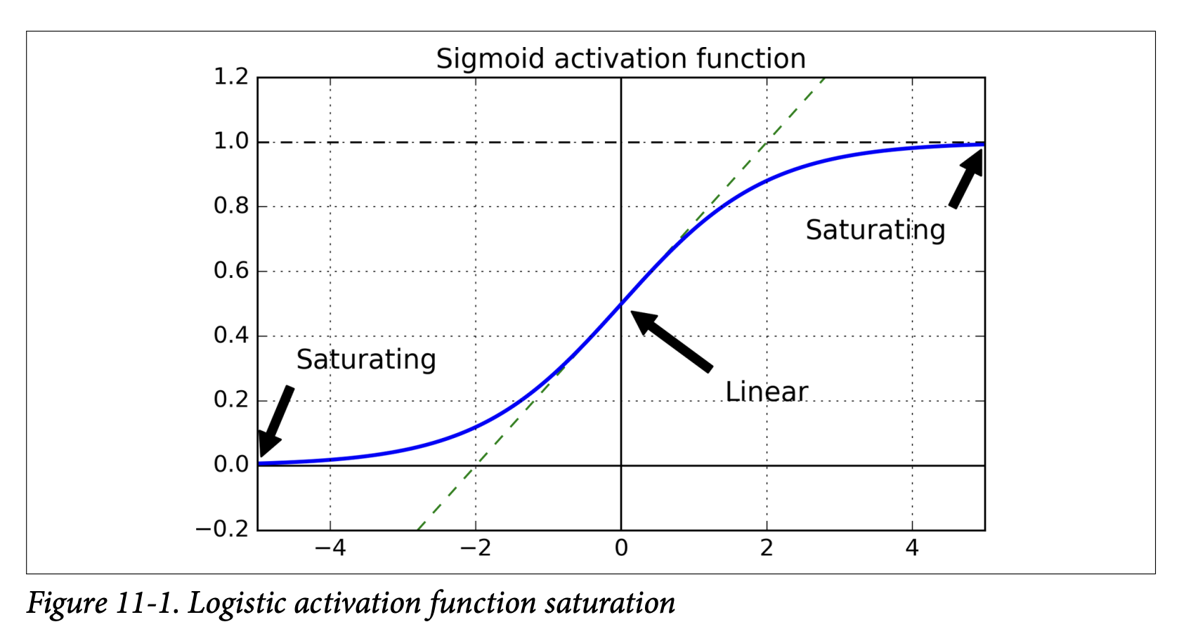
     • In these saturated regions, the derivative of the sigmoid function is extremely close to 0.
     • During backpropagation, when gradients are passed through a saturated sigmoid neuron, they get multiplied by this near-zero derivative, effectively getting squashed.
     • If many layers have saturated sigmoids, the gradient can get diluted to almost nothing by the time it reaches the lower layers.
  2. Traditional Weight Initialization: At the time, weights were often initialized from a normal distribution with mean 0 and standard deviation 1.
  • Variance Imbalance: Glorot and Bengio showed that with this combination (sigmoid activation + standard normal initialization), the variance of the outputs of each layer is much greater than the variance of its inputs.
  • As the signal flows forward, the variance keeps increasing layer by layer. This pushes the inputs to the activation functions of the upper layers into their saturated regions (where derivatives are ~0).
  • The problem is worsened because the logistic function has a mean of 0.5, not 0 (tanh, with mean 0, behaves slightly better).

• The Goal for Proper Signal Flow (Glorot & Bengio’s Insight - Page 333): For a signal (activations forward, gradients backward) to flow properly without dying out or exploding:

  1. The variance of the outputs of each layer should be (roughly) equal to the variance of its inputs.
  2. The gradients should have (roughly) equal variance before and after flowing through a layer in the reverse direction.
  • The analogy (footnote 2) is excellent: a chain of microphone amplifiers. Each needs to be set correctly so your voice comes out clearly at the end, with consistent amplitude through the chain.

  It’s hard to guarantee both conditions 1 & 2 simultaneously unless a layer has an equal number of inputs (fan-in) and outputs/neurons (fan-out).

• Xavier/Glorot Initialization (Equation 11-1, Page 334): Glorot and Bengio proposed a practical compromise for weight initialization that works well:

  • Initialize connection weights randomly.
  • The distribution should have a mean of 0.
  • The variance σ² should depend on fan_in and fan_out: σ² = 1 / fan_avg where fan_avg = (fan_in + fan_out) / 2. (For a uniform distribution between -r and r, r = sqrt(3 / fan_avg)).
  • What this initialization is ultimately trying to achieve: It aims to keep the variance of activations and backpropagated gradients roughly constant across layers, preventing them from vanishing or exploding. It helps the signal propagate properly.
  • This significantly speeds up training and was a key factor in the success of Deep Learning.

• LeCun Initialization (Page 334):

  • An earlier strategy by Yann LeCun (1990s). If you replace fan_avg with just fan_in in Equation 11-1, you get LeCun initialization.
  • Equivalent to Glorot when fan_in = fan_out.

• He Initialization (Kaiming He et al., 2015 - Footnote 3, Page 334):

  • Glorot initialization works well for sigmoid, tanh, and softmax.
  • For ReLU and its variants (which became very popular), a different initialization is needed because ReLU behaves differently (it kills half the activations, which changes variance).
  • He Initialization uses: σ² = 2 / fan_in (For a uniform distribution, r = sqrt(6 / fan_in)).

• Table 11-1 summarizes initialization strategies for different activation functions:

  

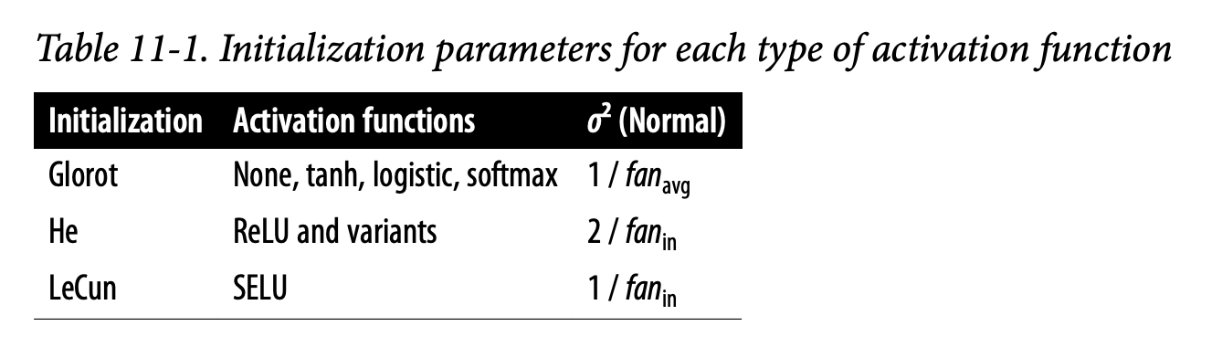
  • Glorot: For None (linear output), tanh, logistic, softmax. Variance 1 / fan_avg.
  • He: For ReLU and variants. Variance 2 / fan_in.
  • LeCun: For SELU (we’ll see this soon). Variance 1 / fan_in.

• Keras Implementation (Page 334):

  • Keras uses Glorot initialization with a uniform distribution by default for its Dense layers.
  • You can change it using kernel_initializer: keras.layers.Dense(10, activation="relu", kernel_initializer="he_normal") keras.layers.Dense(10, activation="relu", kernel_initializer="he_uniform")
  • For He initialization with uniform distribution based on fan_avg (instead of fan_in): he_avg_init = keras.initializers.VarianceScaling(scale=2., mode='fan_avg', distribution='uniform') keras.layers.Dense(..., kernel_initializer=he_avg_init)

These initialization strategies are crucial first steps to combat unstable gradients. They are all trying to set the initial weights to a “sensible” scale so that the signal (activations and gradients) can propagate through many layers without becoming too small or too large too quickly.

Nonsaturating Activation Functions

We’ve seen that a poor choice of activation function (like the traditional sigmoid) combined with older initialization methods was a major cause of unstable gradients. The Glorot & Bengio paper highlighted this.

The Problem with Saturating Activation Functions (like Sigmoid/Tanh):

• Saturation: Functions like sigmoid and tanh “saturate” – their output flattens out and approaches a fixed value (0 or 1 for sigmoid, -1 or 1 for tanh) when the input z becomes very large (positive or negative).
• Vanishing Gradients: In these saturated regions, the derivative of the activation function is extremely close to zero. (Look at Figure 11-1 again for sigmoid).
• Impact on Backpropagation: During backpropagation, the error gradient from the layer above gets multiplied by the local derivative of the activation function. If this derivative is tiny (due to saturation), the gradient being passed back is also tiny.
• Chain Reaction: If many layers have neurons operating in their saturated regions, this “gradient squashing” effect compounds as it goes backward through the network. The gradients reaching the early layers become vanishingly small, and those layers learn very slowly or not at all.

The Solution: Nonsaturating Activation Functions

The insight was to use activation functions that don’t saturate as easily, especially for positive input values.

1. ReLU (Rectified Linear Unit) (Page 335):

   • ReLU(z) = max(0, z)
   • Key Property: For positive values (z > 0), ReLU does not saturate. Its output is just z, and its derivative is 1.
   • This means if a neuron is active (its input z > 0), the gradient can pass through it backward unchanged (multiplied by 1). This greatly helps prevent the vanishing gradient problem for positive activations.
   • It’s also very fast to compute.
   • The “Dying ReLUs” Problem:
     • ReLU is not perfect. If a neuron’s weights get adjusted such that the weighted sum of its inputs (z) becomes negative for all instances in the training set, that neuron will always output 0.
     • Since the derivative of ReLU is 0 for z < 0, no gradient will flow back through this “dead” neuron, and its weights will never be updated again. It effectively dies.
     • This can happen if the learning rate is too large or due to poor initialization.
     • Footnote 4 mentions a dead neuron might sometimes come back to life if neurons in previous layers change their outputs enough to make its input z positive again, but it’s not guaranteed.

2. Leaky ReLU and its Variants (Page 335):

   • Goal: To solve the “dying ReLUs” problem.
   • Leaky ReLU:

     

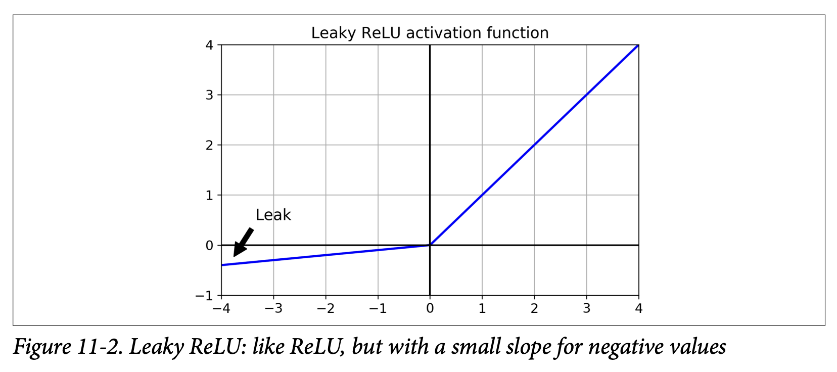
     LeakyReLU_α(z) = max(αz, z)
     • α (alpha) is a small hyperparameter (e.g., 0.01 or 0.2) that defines the slope for z < 0.
     • What it’s ultimately trying to achieve: It allows a small, non-zero gradient to flow back even when the unit is not active (i.e., z < 0). This ensures the neuron never truly “dies” – it can always recover.
     • A 2015 paper (footnote 5) found that leaky variants always outperformed strict ReLU, and a larger “leak” (α = 0.2) was better than a small one (α = 0.01).
   • Randomized Leaky ReLU (RReLU): α is picked randomly from a given range during training and fixed to an average value during testing. Acted as a regularizer.
   • Parametric Leaky ReLU (PReLU): α is learned during training (it becomes another parameter of the network, updated by backpropagation) instead of being a fixed hyperparameter. Reported to outperform ReLU on large image datasets but risks overfitting on smaller ones.

3. ELU (Exponential Linear Unit) (Page 336):

   • Proposed in a 2015 paper by Clevert et al. (footnote 6).
   • Equation 11-2 & Figure 11-3:

     

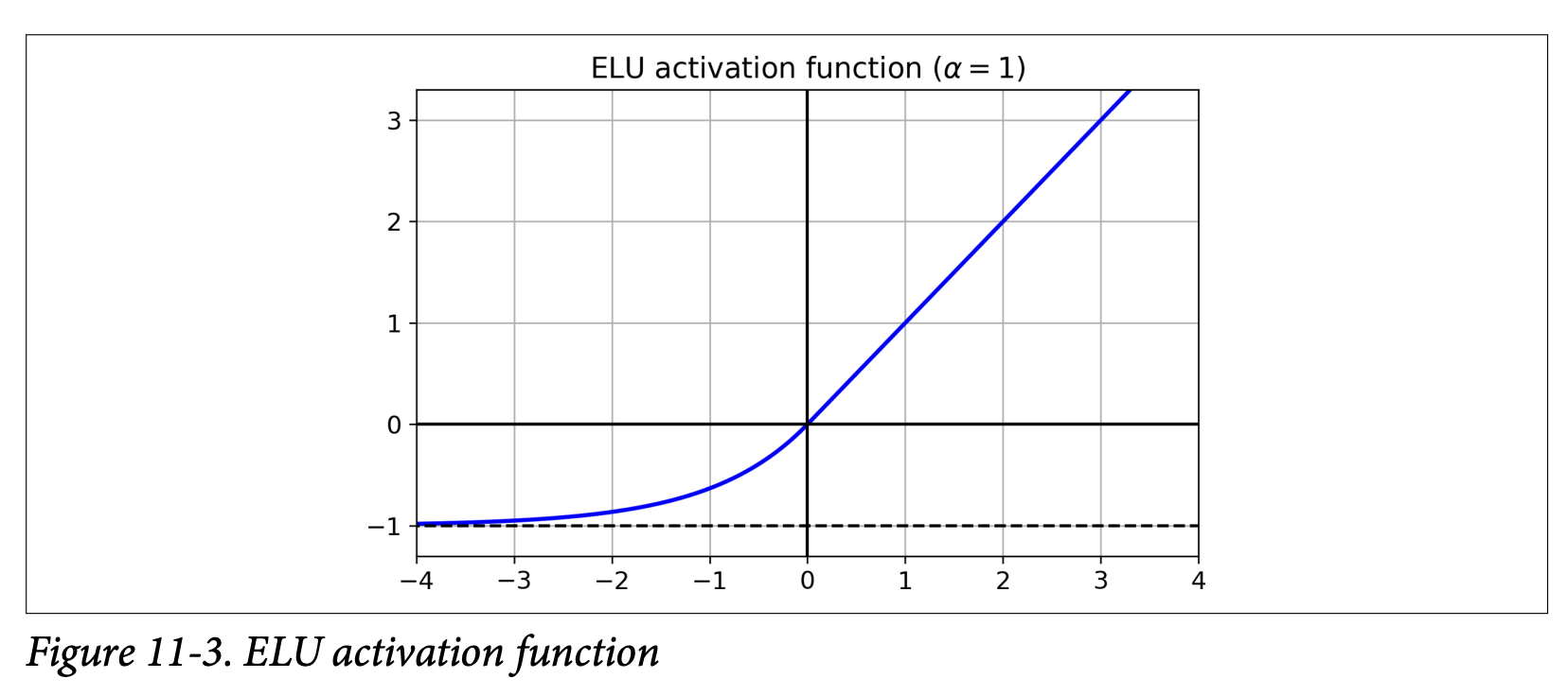
     ELU_α(z) = { α(exp(z) - 1) if z < 0 } { z if z ≥ 0 }
   • Reported to outperform all ReLU variants in their experiments: reduced training time and better test set performance.
   • Key Differences/Advantages over ReLU (Page 337):
     1. Takes on negative values when z < 0: This allows the units to have an average output closer to 0, which can help alleviate the vanishing gradients problem (similar to how tanh is sometimes better than sigmoid because its outputs are centered around 0). The hyperparameter α defines the value ELU approaches for large negative z (usually α=1).
     2. Nonzero gradient for z < 0: Avoids the dying neurons problem. The derivative for z<0 is α*exp(z).
     3. Smooth everywhere (if α=1): Including around z=0. This helps Gradient Descent converge faster as it doesn’t “bounce” as much around z=0 compared to ReLU/Leaky ReLU whose slope changes abruptly.
   • Main Drawback: Slower to compute than ReLU (due to the exp(z) function). However, its faster convergence rate during training often compensates for this. At test time, an ELU network will be slower than a ReLU network.

4. SELU (Scaled ELU) (Page 337):

   • Introduced in a 2017 paper by Klambauer et al. (footnote 7).
   • A scaled variant of ELU.
   • Amazing Property: Self-Normalization! If you build a network composed exclusively of a stack of dense layers, and all hidden layers use SELU activation, and a few other conditions are met, the network will self-normalize.
     • What self-normalization achieves: The output of each layer will tend to preserve a mean of 0 and standard deviation of 1 during training. This solves the vanishing/exploding gradients problem!
     • SELU often significantly outperforms other activation functions for such deep, dense networks.
   • Conditions for Self-Normalization:
     1. Input features must be standardized (mean 0, std dev 1).
     2. Every hidden layer’s weights must be initialized with LeCun normal initialization (in Keras: kernel_initializer="lecun_normal").
     3. Network architecture must be sequential. Does not guarantee self-normalization for non-sequential architectures (like RNNs or networks with skip connections like Wide & Deep).
     4. The paper guarantees it if all layers are dense, but some researchers note it can improve performance in CNNs too.

• Which Activation Function to Use for Hidden Layers? (General Guideline - Lizard Icon, page 338):

  • General Order of Preference: SELU > ELU > Leaky ReLU (and its variants) > ReLU > tanh > logistic.
  • If network architecture prevents self-normalization (e.g., RNNs, skip connections): ELU might perform better than SELU (since SELU isn’t smooth at z=0).
  • Runtime Latency is Critical: Leaky ReLU might be preferred (simpler to compute than ELU/SELU).
  • Simplicity/Don’t want to tune α: Use default α values (Keras uses 0.3 for Leaky ReLU).
  • Spare Time/Compute for CV: Evaluate RReLU (if overfitting) or PReLU (if huge training set).
  • Absolute Speed Priority: ReLU is the most used, so many libraries and hardware have specific optimizations for it. It might still be the best choice if raw speed is paramount.

• Keras Implementation (Page 338):

  • Leaky ReLU: Add a keras.layers.LeakyReLU(alpha=0.2) layer after the Dense layer (if the Dense layer doesn’t have an activation specified).

    model.add(keras.layers.Dense(10, kernel_initializer="he_normal")) # No activation here
    model.add(keras.layers.LeakyReLU(alpha=0.2))
    

  • PReLU: keras.layers.PReLU() (can be added similarly).
  • SELU: Set directly in the Dense layer: keras.layers.Dense(10, activation="selu", kernel_initializer="lecun_normal")

Key Takeaway from this Section: The choice of activation function is critical for mitigating unstable gradients in deep networks.

• Saturating functions (sigmoid, tanh) are generally problematic for deep hidden layers due to vanishing gradients when neurons saturate.
• ReLU was a big step forward because it doesn’t saturate for positive inputs, but it can suffer from “dying neurons.”
• Leaky ReLU, PReLU, ELU address the dying ReLU problem by allowing a small gradient for negative inputs. ELU also offers smoothness and outputs closer to zero mean.
• SELU offers self-normalization under specific conditions, often leading to the best performance for deep stacks of dense layers.
• What all these newer activation functions are ultimately trying to achieve: Maintain a healthy flow of gradients during backpropagation, allowing all layers in a deep network to learn effectively.

This understanding of activation functions and their impact on gradients, combined with proper weight initialization, forms the first line of defense against the vanishing/exploding gradients problem.

Batch Normalization - The Concept

Even with good initialization and activation functions, the vanishing/exploding gradients problem might not be completely solved, or it might reappear during training as weights get updated.

• The Problem Batch Normalization (BN) Addresses:

  • Internal Covariate Shift: As the parameters of preceding layers change during training, the distribution of each layer’s inputs also changes. This makes it harder for the current layer to learn, as it’s constantly adapting to a moving target.
  • Vanishing/Exploding Gradients (still a concern).

• Batch Normalization (BN) - Proposed by Ioffe and Szegedy (2015 - Footnote 8):

  • What it is: A technique that adds an operation in the model, typically just before or after the activation function of each hidden layer.
  • What it does at each layer during training (for each mini-batch):
    1. Zero-centers and normalizes its inputs (makes them have mean 0 and standard deviation 1).
    2. Then, it scales and shifts the result using two new learnable parameter vectors per layer:
       • γ (gamma): for scaling.
       • β (beta): for shifting.
  • What Batch Normalization is ultimately trying to achieve (the high-level goals):
    1. Reduce Internal Covariate Shift: By normalizing the inputs to each layer, it ensures that the distribution of these inputs is more stable throughout training, making it easier for each layer to learn.
    2. Combat Vanishing/Exploding Gradients: By keeping the inputs to activation functions in a more controlled range (around mean 0, std dev 1 before scaling/shifting), it helps prevent them from saturating (for sigmoid/tanh) or dying (for ReLU, by potentially shifting inputs to be positive more often).
    3. Allow higher learning rates: Training becomes more stable, often permitting the use of larger learning rates, which speeds up convergence.
    4. Act as a regularizer: It adds a bit of noise to each layer’s inputs (due to mini-batch statistics varying), which can have a slight regularizing effect, sometimes reducing the need for other regularization like dropout.
    5. Reduce sensitivity to weight initialization.

• How BN Works - The Algorithm (Equation 11-3, Page 339): For each input feature (or activation from a previous neuron) within a mini-batch B:

  1. μ_B = (1/m_B) * Σᵢ x⁽ⁱ⁾: Calculate the mean (μ_B) of that input feature over the current mini-batch B (which has m_B instances).
  2. σ_B² = (1/m_B) * Σᵢ (x⁽ⁱ⁾ - μ_B)²: Calculate the variance (σ_B²) of that input feature over the current mini-batch.
  3. x̂⁽ⁱ⁾ = (x⁽ⁱ⁾ - μ_B) / sqrt(σ_B² + ε): Normalize the input x⁽ⁱ⁾ for each instance. ε (epsilon) is a small smoothing term to avoid division by zero (e.g., 10⁻⁵). Now x̂⁽ⁱ⁾ has mean ~0 and std dev ~1 over this mini-batch.
  4. z⁽ⁱ⁾ = γ ⊗ x̂⁽ⁱ⁾ + β: Scale (γ) and shift (β) the normalized input.
     • γ (gamma) and β (beta) are learnable parameters for this BN layer (one γ and one β per input feature to the layer). They are learned via backpropagation just like weights and biases of dense layers.
     • What γ and β are ultimately trying to achieve: They allow the network to learn the optimal scale and mean for the inputs to the next layer. While the previous steps normalize to mean 0 / std dev 1, maybe the next activation function performs better if its inputs have, say, mean 0.5 and std dev 2. γ and β let the network learn this. If γ = sqrt(σ_B² + ε) and β = μ_B, the BN layer effectively undoes the normalization for that batch.

• BN at Test Time (Inference) (Page 340):

  • During training, μ_B and σ_B are computed per mini-batch.
  • At test time, you might be making predictions for individual instances, so there’s no mini-batch to compute a mean/std dev from. Even with a batch, it might be too small or not representative.
  • Solution: During training, BN layers estimate the “final” population mean μ and standard deviation σ for each input feature using an exponential moving average of the mini-batch μ_B’s and σ_B’s.
  • At test time, these final μ and σ are used in step 3 instead of batch-specific μ_B and σ_B. The learned γ and β are always used.
  • Keras handles this automatically.

• Benefits Demonstrated by Ioffe and Szegedy (Page 340):

  • BN considerably improved all deep networks they experimented with.
  • Huge improvement on ImageNet classification.
  • Vanishing gradients problem strongly reduced, allowing use of saturating activations like tanh/sigmoid.
  • Less sensitive to weight initialization.
  • Able to use much larger learning rates, significantly speeding up learning.
  • Acts as a regularizer, reducing need for other methods like dropout.

• Complexity and Runtime Penalty (Page 341):

  • BN adds complexity to the model.
  • There’s a runtime penalty during inference due to extra computations at each layer.
  • Optimization: It’s often possible to fuse the BN layer with the preceding Dense layer after training. The weights and biases of the Dense layer are updated to directly produce outputs of the appropriate scale and offset, effectively incorporating the BN operation. TFLite’s optimizer can do this automatically.
  • Training Time (Wall Clock): Although each epoch takes longer with BN, convergence is much faster (fewer epochs needed), so overall “wall clock” training time is usually shorter.

(Page 341-344: Implementing Batch Normalization with Keras)

• Simple Implementation:

  • Add a keras.layers.BatchNormalization() layer before or after each hidden layer’s activation function.
  • Optionally, add a BN layer as the very first layer (after Flatten, if using Flatten). If you do this, you might not need to standardize your input data with StandardScaler, as the BN layer will handle normalization (approximately, as it uses mini-batch stats).
  • Example with BN after activation (page 342):

    model = keras.models.Sequential([
        keras.layers.Flatten(input_shape=[28, 28]),
        keras.layers.BatchNormalization(), # As first layer
        keras.layers.Dense(300, activation="elu", kernel_initializer="he_normal"),
        keras.layers.BatchNormalization(), # After first hidden layer's activation
        keras.layers.Dense(100, activation="elu", kernel_initializer="he_normal"),
        keras.layers.BatchNormalization(), # After second hidden layer's activation
        keras.layers.Dense(10, activation="softmax")
    ])
    

  • For shallow networks, BN might not have a huge impact, but for deeper ones, it can be a game-changer.

• Parameters Added by BN Layer (Page 342):

  • Each BN layer adds 4 parameters per input feature it processes:
    1. γ (gamma - scale): Trainable (learned by backprop).
    2. β (beta - shift): Trainable.
    3. μ (moving_mean): Non-trainable (estimated using moving average).
    4. σ (moving_variance): Non-trainable (estimated using moving average).
  • So, if a BN layer receives 784 inputs, it adds 4 * 784 = 3136 parameters. 2 * 784 are trainable (γ, β), 2 * 784 are non-trainable (μ, σ).

• BN Before or After Activation? (Page 343):

  • The original BN paper suggested adding BN before the activation function. The example above added it after.
  • There’s some debate; what’s preferable seems to depend on the task and dataset. Experiment to see what works best.
  • To add BN before activation:
    1. Remove the activation from the Dense layer (activation=None or just omit it).
    2. Add the BatchNormalization layer.
    3. Add an keras.layers.Activation("elu") layer separately.
    4. Also, since BN includes a shift parameter β per input, you can remove the bias term from the preceding Dense layer by setting use_bias=False. This is slightly more efficient.

    model.add(keras.layers.Dense(300, kernel_initializer="he_normal", use_bias=False))
    model.add(keras.layers.BatchNormalization())
    model.add(keras.layers.Activation("elu"))
    

• BatchNormalization Hyperparameters (Page 343):

  • momentum: Used for updating the exponential moving averages for μ and σ. Given new batch stats v_batch, running average v̂ is updated as: v̂ ← v̂ * momentum + v_batch * (1 - momentum).
    • A good value is typically close to 1 (e.g., 0.9, 0.99, 0.999). More 9s for larger datasets/smaller mini-batches. Default is 0.99.
  • axis: Determines which axis should be normalized. Defaults to -1 (last axis).
    • For a Dense layer, inputs are usually (batch_size, features). axis=-1 normalizes each feature independently across the batch.
    • If BN is applied to 3D inputs like (batch_size, height, width) (e.g., before Flatten, or in CNNs), axis=-1 would normalize along the width dimension. If you want to normalize each of the height*width pixels independently, you might set axis=[1,2].

• call() Method and training Argument (Page 344):

  • The BatchNormalization layer’s call() method has a training argument.
  • model.fit() automatically sets this to True during training (so BN uses mini-batch stats and updates moving averages).
  • model.evaluate() and model.predict() automatically set it to False (so BN uses the final moving averages).
  • This is important if you write custom layers that need to behave differently during training vs. inference.

• BN as a Standard (Page 344):

  • BN became so popular that it’s often assumed to be used after every (or most) layers in deep networks, sometimes even omitted in diagrams.
  • However, recent research (e.g., “Fixup Initialization” by Zhang et al., 2019 - footnote 11) has shown it’s possible to train very deep networks without BN by using novel weight initialization techniques. This is bleeding-edge, so for now, BN remains a very strong default.

Key Takeaway for Batch Normalization: BN is a powerful technique that normalizes the inputs to each layer during training, then scales/shifts them with learnable parameters.

• Ultimately, it aims to:
  • Stabilize and speed up training (allowing higher learning rates).
  • Reduce the vanishing/exploding gradient problem.
  • Make the network less sensitive to weight initialization.
  • Provide a slight regularization effect. It’s a very common and effective component in modern deep neural networks.

Great! Batch Normalization is indeed a very impactful technique.

Gradient Clipping

While Batch Normalization helps with unstable gradients generally, sometimes gradients can still become excessively large, especially in certain types of networks like Recurrent Neural Networks (RNNs, Chapter 15). This is the exploding gradients problem.

• The Problem: If gradients become huge, the parameter updates during Gradient Descent will also be huge (θ ← θ - η * large_gradient). This can cause the algorithm to overshoot the optimal solution wildly, leading to divergence (loss goes to infinity) or very unstable training.

• Gradient Clipping - The Technique:

  • A popular technique to mitigate exploding gradients.
  • What it’s ultimately trying to achieve: To prevent the gradients from becoming too large by imposing a threshold on them during backpropagation. If a gradient exceeds this threshold, it’s “clipped” (scaled down) to the threshold value.
  • This is most often used in RNNs, as Batch Normalization can be tricky to apply effectively in those architectures. For other types of networks (like the MLPs we’ve been discussing), Batch Normalization is usually sufficient to handle unstable gradients.

• Implementing Gradient Clipping in Keras: It’s done by setting an argument when creating an optimizer. Keras supports two main types of clipping:

  1. Clipping by Value: optimizer = keras.optimizers.SGD(clipvalue=1.0)

     • This will clip every component (each partial derivative) of the gradient vector to be within a specific range. In this example, between -1.0 and +1.0.
     • So, if any ∂Loss/∂wᵢⱼ is, say, 3.5, it will be clipped to 1.0. If it’s -2.0, it will be clipped to -1.0.
     • Caveat: Clipping each component individually may change the orientation (direction) of the overall gradient vector. For instance, if the original gradient was [0.9, 100.0] (pointing mostly along the second axis), after clipping by value to 1.0, it becomes [0.9, 1.0] (pointing roughly diagonally).
     • Despite this, it often works well in practice. The clipvalue is a hyperparameter you can tune.

  2. Clipping by Norm: optimizer = keras.optimizers.SGD(clipnorm=1.0)

     • This method ensures that the direction of the gradient vector is preserved.
     • It calculates the ℓ₂ norm of the entire gradient vector ||∇Loss||₂.
     • If this norm is greater than the clipnorm threshold (e.g., 1.0), the entire gradient vector is scaled down so that its norm equals the threshold. gradient ← gradient * (clipnorm / ||gradient||₂)
     • For example, if clipnorm=1.0 and the original gradient is [0.9, 100.0] (whose norm is sqrt(0.9² + 100.0²) ≈ 100.004), it will be scaled down to something like [0.00899964, 0.9999595]. The direction is preserved, but the magnitude is reduced to 1.0.
     • This can be gentler as it doesn’t distort the gradient direction, but it might almost eliminate components that were originally small if one component was huge.

• When to Use:

  • If you observe that gradients are exploding during training (you can track gradient norms using TensorBoard, for example, or just see your loss skyrocket), you might want to try gradient clipping.
  • Experiment with both clipping by value and clipping by norm, and different threshold values, to see which works best for your specific problem and network.

Key Takeaway for Gradient Clipping: It’s a straightforward technique primarily used to prevent the exploding gradients problem by limiting the maximum size of the gradients used in the parameter updates. While BN is often preferred for feedforward networks, clipping is a valuable tool, especially for RNNs.

This technique directly addresses one of the “pain points” of training deep networks. Next, the chapter moves on to strategies for dealing with another major challenge: not having enough labeled training data, by discussing Reusing Pretrained Layers (Transfer Learning).

Sounds good! Gradient clipping is indeed a practical fix for a very real problem.

Now, let’s move on to a very powerful and widely used set of techniques for training deep neural networks, especially when you don’t have massive amounts of labeled data: Reusing Pretrained Layers, which is the core idea behind Transfer Learning (Pages 345-349).

Reusing Pretrained Layers - The Concept of Transfer Learning

• The Problem: Training a very large Deep Neural Network (DNN) from scratch generally requires a huge amount of training data. What if you don’t have that much data for your specific task?

• The Solution: Transfer Learning

  • Core Idea: It’s generally not a good idea to train a very large DNN from scratch if you can avoid it. Instead, you should almost always try to find an existing neural network that was trained on a large dataset to accomplish a task similar to yours. Then, you reuse the lower layers of this pretrained network for your own new model.
  • What transfer learning is ultimately trying to achieve:
    1. Speed up training considerably: Your model doesn’t have to learn low-level features from scratch.
    2. Require significantly less training data for your specific task: The pretrained layers have already learned general features from a large dataset, which are often useful for your new task.
    3. Often achieve better performance than training from scratch, especially with limited data.

• Why it Works (Hierarchical Feature Learning):

  • As we discussed in Chapter 10 (and mentioned in this chapter on page 323), deep neural networks learn features in a hierarchical fashion.
    • Lower layers (closer to the input) tend to learn low-level features (e.g., edges, corners, simple textures in images; basic phonetic sounds in speech). These low-level features are often generic and useful across many different tasks.
    • Upper hidden layers learn more complex, task-specific features by combining the low-level features from earlier layers (e.g., parts of objects like “wheel” or “eye” in images; words or phrases in speech).
    • Output layer learns to combine these high-level features to make the final prediction for the original task.

• Applying Transfer Learning (Figure 11-4):

  

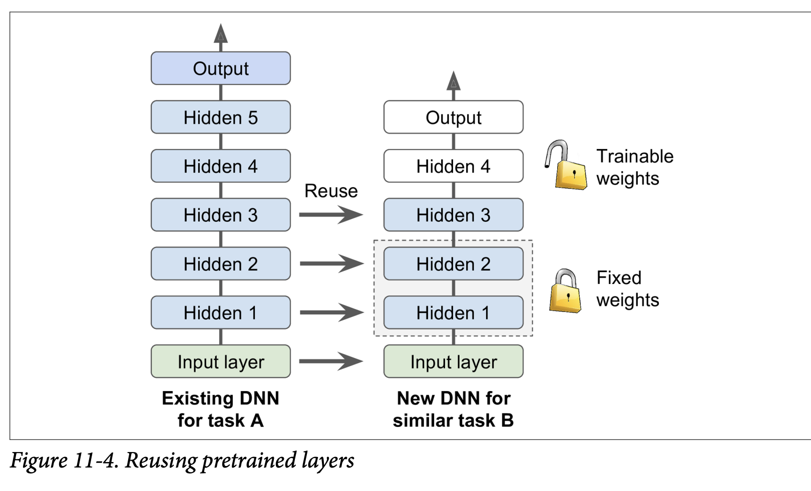
  • Suppose you have a DNN (Model A) pretrained on a large dataset for a general task (e.g., classifying images into 100 categories like animals, plants, vehicles).
  • You now want to train a DNN (Model B) for a new, more specific task (e.g., classifying only specific types of vehicles), and you have limited data for this new task.
  • Steps:
    1. Reuse Lower Layers: Take the lower layers from Model A (which learned general features) and use them as the initial layers for your Model B.
    2. Replace or Retrain Upper Layers: The upper hidden layers and the output layer of Model A are more specific to its original task.
       • The output layer of Model A must usually be replaced because it’s likely not useful for Model B (e.g., different number of classes, different types of outputs).
       • The upper hidden layers of Model A might be useful, or they might be too specific. You need to decide how many of these to reuse.
    3. Train Model B: Train your new model (with the reused lower layers and new/modified upper layers) on your smaller dataset for Task B.

• Preprocessing Input (Bird Icon, page 346):

  • If the input data for your new task (Task B) doesn’t have the same size/format as the data Model A was trained on, you’ll usually need to add a preprocessing step to resize/reformat your new data to match what the pretrained layers expect.
  • Transfer learning works best when the inputs for the new task have similar low-level features to the original task.

• How Many Layers to Reuse? (Page 346 & Snake Icon, page 347):

  • The more similar the tasks are, the more layers you can (and probably should) reuse. For very similar tasks, you might reuse all hidden layers and just replace the output layer.
  • Strategy for Fine-Tuning:
    1. Freeze Reused Layers Initially: When you first start training Model B, it’s often a good idea to freeze the weights of the reused layers (make them non-trainable so Gradient Descent won’t modify them).
       • Why? Your new output layer (and any new upper hidden layers) will have randomly initialized weights. If you train everything at once, the large error gradients from these random layers could propagate back and wreck the carefully tuned weights of the pretrained lower layers.
       • Train the model for a few epochs with the reused layers frozen. This allows the new layers to learn reasonable weights without damaging the pretrained ones.
    2. Unfreeze Some Layers and Fine-Tune: After the new layers have settled a bit, you can unfreeze some or all of the reused layers (typically starting with the upper ones) and continue training. This allows backpropagation to fine-tune these reused weights for your specific new task.
       • Reduce Learning Rate: When you unfreeze reused layers, it’s usually beneficial to use a much smaller learning rate. This is to make only small adjustments to the already good pretrained weights, rather than drastically changing them.
    3. Iterate: If you still can’t get good performance and have little data, try dropping some of the top reused hidden layers and freezing all remaining reused layers again. If you have plenty of training data, you might try replacing the top hidden layers or even adding more new hidden layers on top of the reused ones.

• Transfer Learning with Keras (Page 347-348): The book gives an example:

  • Model A: Trained on Fashion MNIST for 8 classes (excluding sandal and shirt). Achieved >90% accuracy.
  • Task B: Binary classifier for shirt (positive) vs. sandal (negative). Small dataset (200 labeled images).
  • Training a new model (same architecture as A) from scratch on Task B gets ~97.2% accuracy. Can transfer learning do better?
  1. Load Model A and Create Model B: model_A = keras.models.load_model("my_model_A.h5") model_B_on_A = keras.models.Sequential(model_A.layers[:-1]) # Reuse all layers except output model_B_on_A.add(keras.layers.Dense(1, activation="sigmoid")) # New binary output layer
  2. Cloning (Important!):
     • The code above makes model_B_on_A share layers with model_A. If you train model_B_on_A, it will change the weights in model_A as well!
     • To avoid this, clone model_A first if you want to keep model_A intact: model_A_clone = keras.models.clone_model(model_A) model_A_clone.set_weights(model_A.get_weights()) Then build model_B_on_A using model_A_clone.layers[:-1].
  3. Freeze Reused Layers: for layer in model_B_on_A.layers[:-1]: layer.trainable = False model_B_on_A.compile(...) (You must recompile after changing trainable status).
  4. Train the New Layer(s): history = model_B_on_A.fit(X_train_B, y_train_B, epochs=4, ...) (Train for a few epochs).
  5. Unfreeze and Fine-Tune: for layer in model_B_on_A.layers[:-1]: layer.trainable = True optimizer = keras.optimizers.SGD(learning_rate=1e-4) # Use a lower learning rate model_B_on_A.compile(..., optimizer=optimizer, ...) history = model_B_on_A.fit(X_train_B, y_train_B, epochs=16, ...)
  • Result: The example shows the transfer learning model achieved 99.25% accuracy, reducing the error rate from 2.8% (model from scratch) to ~0.7% – a factor of four improvement!
  • Caveat (“Torturing the Data”): The author admits to “cheating” a bit by trying many configurations to find one that showed a strong improvement for this specific example. Transfer learning doesn’t always give such dramatic gains for small dense networks (they learn few, specific patterns). It works best with deep convolutional neural networks (CNNs) which learn more general feature detectors, especially in lower layers. (This will be revisited in Chapter 14).

(Page 349-350: Unsupervised Pretraining)

What if you want to tackle a complex task, you don’t have much labeled data, AND you can’t find a pretrained model trained on a similar task?

• The Idea: If you can gather plenty of unlabeled training data (which is often cheap and easy), you can use it to train an unsupervised model first.
  • Examples of unsupervised models: Autoencoders, Generative Adversarial Networks (GANs) (Chapter 17).
• The Process (Figure 11-5, page 350):
  1. Train an unsupervised model (e.g., an autoencoder) on your large unlabeled dataset.
     • What this unsupervised training is trying to achieve: The lower layers of this model will learn to detect useful low-level features and patterns present in your unlabeled data.
  2. Reuse the lower layers of this pretrained unsupervised model.
  3. Add an output layer suitable for your actual supervised task on top.
  4. Fine-tune this final network using your small amount of labeled training data.
• Historical Significance: This technique (often with Restricted Boltzmann Machines - RBMs, Appendix E) was crucial for the revival of neural networks and the success of Deep Learning from 2006 until around 2010. After the vanishing gradients problem was better understood and mitigated (with better initializers, activations, etc.), purely supervised training of DNNs became more common when large labeled datasets were available.
• Modern Relevance: Unsupervised pretraining (now typically using autoencoders or GANs) is still a very good option when:
  • You have a complex task.
  • No similar pretrained model is available.
  • You have little labeled data but plenty of unlabeled data.
• Greedy Layer-Wise Pretraining (Old Technique - Figure 11-5, top part):
  • In the early days, training deep models was very hard. So, people would train one unsupervised layer (e.g., RBM) at a time, freeze it, add another on top, train that new layer, freeze it, and so on.
  • Nowadays, things are simpler: people generally train the full unsupervised model (e.g., a deep autoencoder) in one shot (Figure 11-5, starting at step three).

(Page 350-351: Pretraining on an Auxiliary Task)

One last option if you don’t have much labeled data for your main task:

• The Idea: Find an auxiliary task for which you can easily obtain or generate a lot of labeled training data.
• Train a first neural network on this auxiliary task.
• Reuse the lower layers of this network (which learned feature detectors relevant to the auxiliary task) for your actual main task.
• What this is ultimately trying to achieve: Hope that the features learned for the auxiliary task are also somewhat relevant and useful for your main task.
• Examples:
  • Face Recognition: If you have few pictures of each specific person you want to recognize (main task), you could first gather lots of pictures of random people from the web and train a network to detect whether two different pictures feature the same person (auxiliary task – a “Siamese network” setup). This network would learn good general face feature detectors.
  • Natural Language Processing (NLP): Download millions of text documents. Automatically generate labeled data by, for example, randomly masking out some words and training a model to predict the missing words (this is a form of self-supervised learning). A model that performs well on this task (like BERT or GPT) learns a lot about language structure. Its lower layers can then be reused and fine-tuned for a specific NLP task (like sentiment analysis) for which you might have less labeled data. (More in Chapter 15).
• Self-Supervised Learning (Bird Icon, page 351): When you automatically generate labels from the data itself (like masking words), it’s called self-supervised learning. Since no human labeling is needed, it’s often classified as a form of unsupervised learning.

Key Takeaway for Reusing Layers/Pretraining: These techniques are all about leveraging knowledge learned from one task/dataset to help with another, especially when labeled data for the target task is scarce.

• Transfer Learning: Reuse layers from a model trained on a similar supervised task.
• Unsupervised Pretraining: Train on unlabeled data first to learn general features, then fine-tune for a supervised task.
• Pretraining on an Auxiliary Task: Train on a related task where labeled data is abundant, then transfer.

These are powerful strategies to build effective deep learning models more efficiently.

Faster Optimizers

The book states, “Training a very large deep neural network can be painfully slow.” So far, we’ve seen four ways to speed up training (and potentially reach a better solution):

1. Applying a good initialization strategy for connection weights (Glorot, He).
2. Using a good activation function (ReLU, ELU, SELU).
3. Using Batch Normalization.
4. Reusing parts of a pretrained network (transfer learning).

Another huge speed boost comes from using a faster optimizer than the regular (Mini-batch) Gradient Descent optimizer we’ve mostly considered so far. This section presents the most popular advanced optimization algorithms.

What all these faster optimizers are ultimately trying to achieve: They aim to converge to a good solution more quickly than standard Gradient Descent by being smarter about the direction and size of the steps taken in the parameter space to minimize the loss function. They often do this by incorporating information about past gradients or by adapting the learning rate for different parameters.*

1. Momentum Optimization (Page 351-352):

   • Proposed by Boris Polyak in 1964.
   • Analogy: Imagine a bowling ball rolling down a gentle slope. It starts slowly but picks up momentum and reaches a terminal velocity. Regular Gradient Descent (GD) just takes small, regular steps, like someone carefully walking down.
   • Core Idea: Momentum optimization cares a great deal about previous gradients.
     • At each iteration, it subtracts the current local gradient from a momentum vector m.
     • It then updates the weights θ by adding this momentum vector m.
     • The gradient is used for acceleration, not directly for speed.
   • Friction Mechanism: To prevent momentum from growing too large, a hyperparameter β (beta), called the momentum, is introduced (between 0 for high friction and 1 for no friction). A typical value is 0.9.
   • Equation 11-4: Momentum algorithm
     1. m ← βm - η∇_θJ(θ) (Update momentum vector: previous momentum is decayed by β, and then the current negative gradient scaled by learning rate η is added/subtracted).
     2. θ ← θ + m (Update parameters using the momentum vector).
   • Benefits:
     • Faster Convergence: If the gradient remains constant, the terminal velocity (max update size) is η * gradient / (1-β). If β=0.9, this is 10 times faster than standard GD!
     • Escapes Plateaus Faster: Standard GD moves very slowly on flat regions. Momentum helps “roll” through them.
     • Helps with Elongated Bowls: In cost functions that look like elongated bowls (common when input features have different scales and no Batch Norm), GD goes down the steep slope quickly but then slowly navigates the valley. Momentum helps roll down the valley faster.
     • Can Roll Past Local Optima: The momentum can sometimes carry the optimization past small local optima.
   • Drawback (Bird Icon, page 352):
     • May overshoot the minimum, then come back, oscillate a few times before stabilizing. The friction β helps dampen these oscillations.
     • Adds another hyperparameter (β) to tune (though 0.9 often works well).
   • Keras Implementation: Use the SGD optimizer and set its momentum hyperparameter: optimizer = keras.optimizers.SGD(learning_rate=0.001, momentum=0.9)

2. Nesterov Accelerated Gradient (NAG) (Page 353):

   • Proposed by Yurii Nesterov in 1983. Almost always faster than vanilla momentum optimization.
   • Core Idea: Instead of calculating the gradient at the current position θ (like vanilla momentum), NAG calculates the gradient slightly ahead in the direction of the momentum, at θ + βm.
   • Equation 11-5: Nesterov Accelerated Gradient algorithm
     1. m ← βm - η∇_θJ(θ + βm) (Calculate gradient at the “look-ahead” position).
     2. θ ← θ + m
   • Why it’s better (Figure 11-6):

     

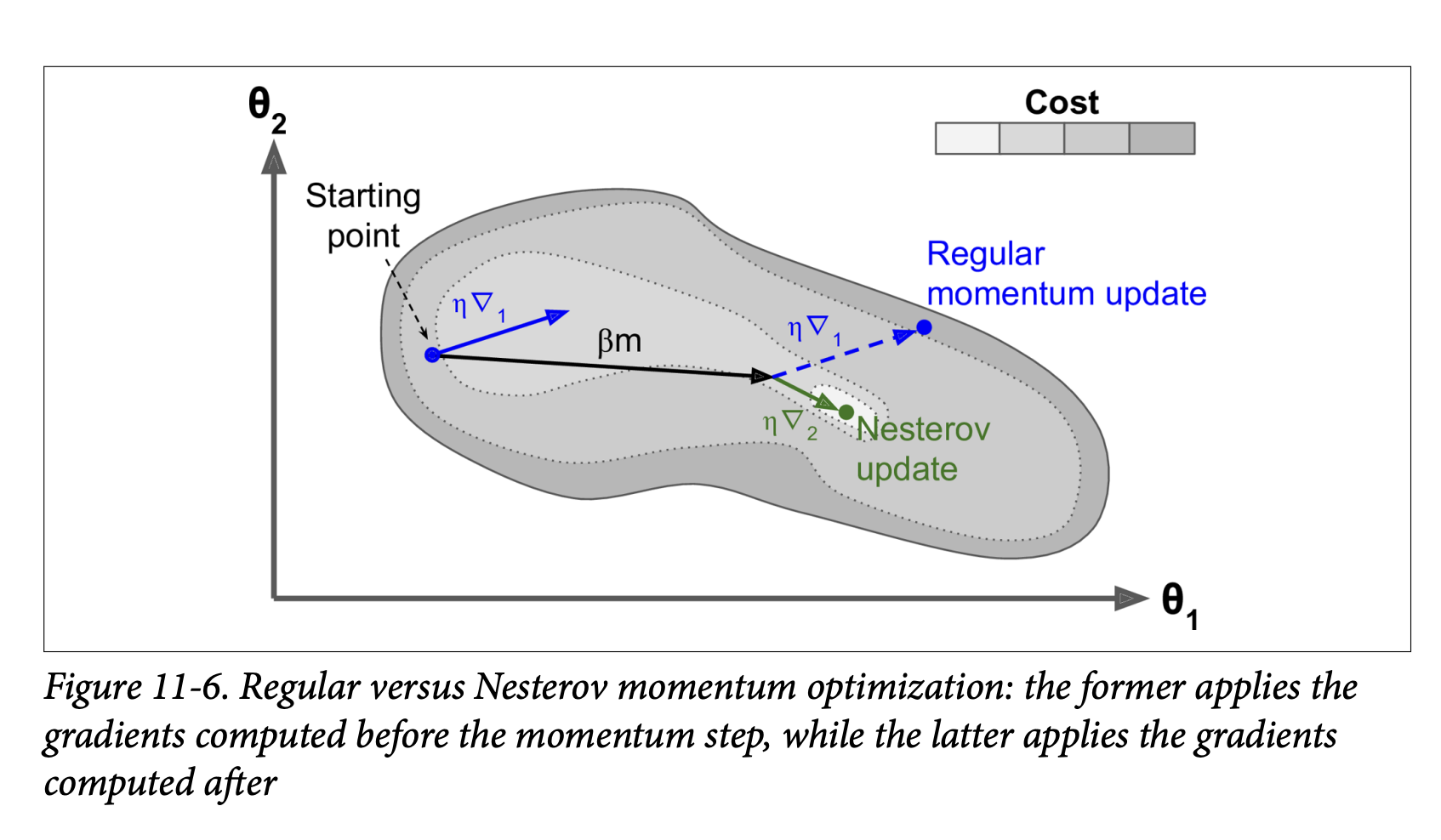
     • The momentum vector m generally points towards the optimum. So, the gradient measured slightly ahead in that direction (∇₂ in the figure) is a more accurate estimate of the “true” gradient towards the optimum than the gradient at the original position (∇₁).
     • When momentum pushes weights across a valley, ∇₁ (original gradient) might continue to push it further across. ∇₂ (look-ahead gradient) will start to push back towards the bottom of the valley sooner. This helps reduce oscillations and converge faster.
   • Keras Implementation: Set nesterov=True in the SGD optimizer: optimizer = keras.optimizers.SGD(learning_rate=0.001, momentum=0.9, nesterov=True)

3. AdaGrad (Adaptive Gradient Algorithm) (Page 354-355):

   • Addresses the “elongated bowl” problem differently. GD goes down steep slopes quickly but then slows down in gentle-sloped valleys. AdaGrad tries to correct its direction earlier to point more towards the global optimum.
   • Core Idea: It scales down the gradient vector along the steepest dimensions (i.e., it “dampens” movement in directions where the gradient has been consistently large). This is an adaptive learning rate method – different learning rates for different parameters.
   • Equation 11-6: AdaGrad algorithm
     1. s ← s + ∇_θJ(θ) ⊗ ∇_θJ(θ) (Accumulate the square of the gradients into vector s. ⊗ is element-wise multiplication. So sᵢ ← sᵢ + (∂J/∂θᵢ)²).
     2. θ ← θ - η ∇_θJ(θ) ⊘ sqrt(s + ε) (⊘ is element-wise division, ε is a small smoothing term to avoid division by zero).
   • How it works:
     • If the cost function is steep along dimension i, (∂J/∂θᵢ)² will be large, so sᵢ will accumulate quickly.
     • In step 2, the update for θᵢ is divided by sqrt(sᵢ + ε). If sᵢ is large, this division scales down the learning rate specifically for θᵢ.
     • So, learning rate decays faster for steep dimensions and slower for dimensions with gentler slopes.
   • Benefits (Figure 11-7): Points updates more directly towards the global optimum. Requires less tuning of the learning rate η.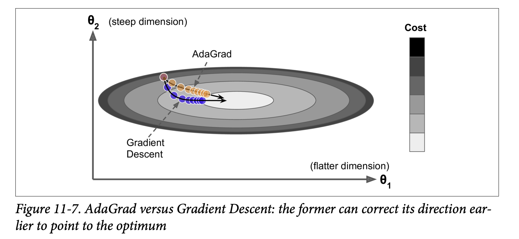

     

   • Drawback: Often stops too early when training neural networks. The learning rate gets scaled down so much (as s keeps accumulating) that the algorithm halts before reaching the global optimum.
   • Keras: keras.optimizers.Adagrad(). Not recommended for deep neural networks due to premature stopping, but understanding it helps with RMSProp and Adam.

4. RMSProp (Root Mean Square Propagation) (Page 355-356):

   • Addresses AdaGrad’s problem of stopping too early.
   • Core Idea: Instead of accumulating all past squared gradients in s, RMSProp accumulates only the gradients from the most recent iterations by using an exponential decay in the first step.
   • Equation 11-7: RMSProp algorithm
     1. s ← βs + (1-β)∇_θJ(θ) ⊗ ∇_θJ(θ) (Exponentially decaying average of squared gradients. β is a decay rate, e.g., 0.9).
     2. θ ← θ - η ∇_θJ(θ) ⊘ sqrt(s + ε) (Same update rule as AdaGrad, using the new s).
   • The decay rate β (typically 0.9) is a new hyperparameter, but the default often works well.
   • Performance: Almost always performs much better than AdaGrad. It was a preferred optimizer until Adam came along.
   • Keras: keras.optimizers.RMSprop(learning_rate=0.001, rho=0.9) (where rho corresponds to β).

5. Adam (Adaptive Moment Estimation) and Nadam (Page 356-358):

   • Adam (Kingma & Ba, 2014 - Footnote 17): Combines the ideas of Momentum optimization and RMSProp.

     • Keeps an exponentially decaying average of past gradients (like momentum, this is the “first moment,” m).
     • Keeps an exponentially decaying average of past squared gradients (like RMSProp, this is the “second moment,” s).

   • Equation 11-8: Adam algorithm

     1. m ← β₁m + (1-β₁)∇_θJ(θ) (Update biased first moment estimate)
     2. s ← β₂s + (1-β₂)∇_θJ(θ) ⊗ ∇_θJ(θ) (Update biased second moment estimate)
     3. m̂ ← m / (1 - β₁ᵗ) (Bias-corrected first moment estimate, t is iteration number)
     4. ŝ ← s / (1 - β₂ᵗ) (Bias-corrected second moment estimate)
     5. θ ← θ - η m̂ ⊘ (sqrt(ŝ) + ε) (Update parameters)

   • Steps 3 & 4 are technical details to correct for the fact that m and s are initialized at 0 and would be biased towards 0 early in training.

   • Hyperparameters:

     • η (learning rate): Typically 0.001.
     • β₁ (momentum decay): Typically 0.9.
     • β₂ (scaling decay for squared gradients): Typically 0.999.
     • ε (smoothing term): Typically 10⁻⁷.

   • Performance: Adam is an adaptive learning rate algorithm, so it often requires less tuning of the learning rate η. Often very easy to use and a good default.

   • Keras: keras.optimizers.Adam(learning_rate=0.001, beta_1=0.9, beta_2=0.999)

   • AdaMax (Variant of Adam - Page 357):

     • Instead of using the ℓ₂ norm (square root of sum of squares) of time-decayed gradients to scale updates (like Adam effectively does via sqrt(ŝ)), AdaMax uses the ℓ∞ norm (the maximum value).
     • Can be more stable than Adam in some cases, but Adam generally performs better.

   • Nadam (Page 358):

     • Adam optimization + Nesterov trick (calculates gradient using the “look-ahead” momentum m̂).
     • Often converges slightly faster than Adam.
     • Timothy Dozat’s report (footnote 19) found Nadam generally outperforms Adam but can sometimes be outperformed by RMSProp.

   • Caveat for Adaptive Optimizers (Scorpion Icon, page 358):

     • Adaptive methods (RMSProp, Adam, Nadam) are often great and converge fast.
     • However, a 2017 paper (Wilson et al. - footnote 20) showed they can generalize poorly on some datasets compared to simpler methods like SGD with Nesterov momentum.
     • Practical Advice: If disappointed by your model’s performance with an adaptive optimizer, try plain Nesterov Accelerated Gradient. Your dataset might be “allergic” to adaptive gradients. Research is ongoing and moving fast.

• Second-Order Partial Derivatives (Hessians - Page 358):

  • All optimizers discussed so far use first-order partial derivatives (Jacobians/gradients).
  • Optimization literature also has algorithms using second-order partial derivatives (Hessians – derivatives of the gradients).
  • These are very hard to apply to DNNs because the number of Hessians is huge (n² per output, where n is number of parameters), so they often don’t fit in memory, and computing them is too slow.

• Training Sparse Models (Sidebar, page 359):

  • If you need a fast model at runtime or one that uses less memory, you might want a sparse model (most parameters are zero).
  • Optimizers discussed produce dense models.
  • Achieving sparsity:
    1. Train as usual, then set tiny weights to zero (pruning). Often doesn’t lead to very sparse models and can degrade performance.
    2. Apply strong ℓ₁ regularization during training (pushes optimizer to zero out weights, like Lasso).
    3. Use tools like TensorFlow Model Optimization Toolkit (TF-MOT), which has pruning APIs.

• Table 11-2: Optimizer Comparison (Page 359): A nice summary table rating convergence speed and quality for SGD, SGD with momentum, Adagrad, RMSProp, Adam, Nadam, AdaMax.

  • SGD: Slow, but can reach good quality.
  • Momentum/NAG: Faster convergence, good quality.
  • Adagrad: Fast convergence, but often stops too early (poor quality for DNNs).
  • RMSProp, Adam, Nadam, AdaMax: Generally fast convergence and good quality. Adam/Nadam are often excellent starting points.

Key Takeaway for Faster Optimizers: Standard Gradient Descent can be slow. Advanced optimizers use techniques like momentum, adaptive learning rates per parameter, or a combination, to navigate the loss landscape more efficiently and converge faster to a good solution. Adam or Nadam are often good defaults, but if they don’t generalize well, try SGD with Nesterov momentum.

This section provides a fantastic toolkit of optimizers beyond basic SGD. They are essential for training deep networks in a reasonable amount of time.

Alright, let’s keep the momentum going! We’ve covered optimizers that try to take smarter steps. Now, let’s talk about how to adjust the size of those steps during training: Learning Rate Scheduling (Pages 359-363).

Learning Rate Scheduling - The Why and How

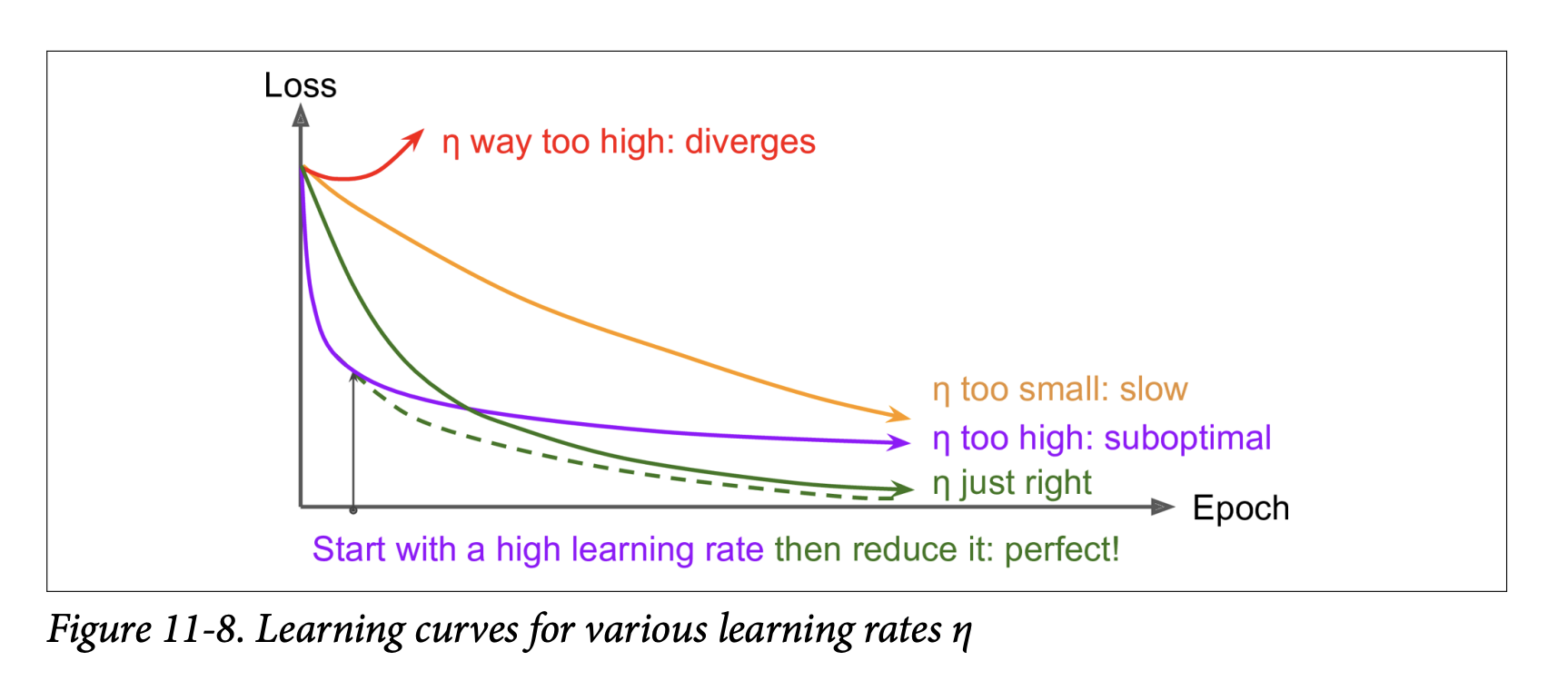
We know that finding a good learning rate η is crucial:

• Too high: Training may diverge (loss explodes).

• Too low: Training converges eventually, but takes a very long time.

• Slightly too high: May make quick initial progress but then dance around the optimum, never settling. (See Figure 11-8).

  

• Finding a Good Constant Learning Rate (Recap from Chapter 10):

  • Train for a few hundred iterations, starting with a very small η and exponentially increasing it.
  • Plot loss vs. η (log scale for η).
  • Pick a learning rate slightly lower than where the loss starts shooting back up.
  • Reinitialize and train with this constant η.

• Doing Better Than a Constant Learning Rate:

  • If you start with a large learning rate and then reduce it once training stops making fast progress, you can often reach a good solution faster than with the single best constant learning rate.
  • These strategies to reduce the learning rate during training are called learning schedules.
  • It can also be beneficial to start with a low learning rate, increase it (warm-up), then drop it again.

What learning rate scheduling is ultimately trying to achieve: To speed up convergence and potentially reach a better final solution by dynamically adjusting the step size of the optimizer during training. Large steps early on can help navigate flat regions or escape poor local minima quickly, while smaller steps later can help fine-tune the solution around the optimum.*

Commonly Used Learning Schedules (Page 360-361):

1. Power Scheduling:

   • η(t) = η₀ / (1 + t/s)ᶜ
     • t: Iteration number.
     • η₀: Initial learning rate.
     • s: A hyperparameter determining how many steps it takes for η to drop significantly.
     • c: Power (typically set to 1).
   • Behavior: Learning rate drops at each step. After s steps, η ≈ η₀ / 2. After another s steps, η ≈ η₀ / 3, then η₀ / 4, etc.
   • Drops quickly at first, then more and more slowly.
   • Requires tuning η₀ and s (and possibly c).
   • Keras Implementation (Easiest - Page 362): Set the decay hyperparameter when creating an SGD optimizer. decay is the inverse of s (and c is assumed to be 1). optimizer = keras.optimizers.SGD(learning_rate=0.01, decay=1e-4) (This means s = 1 / 1e-4 = 10000. So after 10000 steps, η will be roughly 0.01/2).

2. Exponential Scheduling:

   • η(t) = η₀ * 0.1^(t/s)
   • Behavior: Learning rate drops by a factor of 10 every s steps.
   • More aggressive reduction than power scheduling (keeps slashing by a constant factor).
   • Keras Implementation (Page 362):
     • Define a function that takes the current epoch and returns the learning rate:

       def exponential_decay_fn(epoch):
           return 0.01 * 0.1**(epoch / 20)
       # Or a configurable one:
       # def exponential_decay(lr0, s):
       #     def exponential_decay_fn(epoch):
       #         return lr0 * 0.1**(epoch / s)
       #     return exponential_decay_fn
       # exponential_decay_fn = exponential_decay(lr0=0.01, s=20)
       

     • Create a LearningRateScheduler callback and pass it to fit(): lr_scheduler = keras.callbacks.LearningRateScheduler(exponential_decay_fn) history = model.fit(..., callbacks=[lr_scheduler])
     • This updates η at the beginning of each epoch.
     • If you want updates at every step (more frequent), you can write a custom callback.
     • The schedule function can optionally take the current lr as a second argument if it needs to know the previous learning rate.
     • Important if using epoch in schedule function: If you save and then continue training, the epoch argument resets to 0. You might need to set fit()’s initial_epoch argument to avoid this.

3. Piecewise Constant Scheduling:

   • Use a constant η₀ for e₀ epochs, then a smaller η₁ for e₁ epochs, and so on.
   • Can work very well but requires fiddling to find the right sequence of rates and durations.
   • Keras Implementation (Page 363): Use a schedule function with LearningRateScheduler callback, similar to exponential scheduling:

     def piecewise_constant_fn(epoch):
         if epoch < 5: return 0.01
         elif epoch < 15: return 0.005
         else: return 0.001
     

4. Performance Scheduling:

   • Measure validation error every N steps (like early stopping).
   • Reduce η by a factor λ when the error stops dropping.
   • Keras Implementation (Page 363): Use the ReduceLROnPlateau callback. lr_scheduler = keras.callbacks.ReduceLROnPlateau(factor=0.5, patience=5)
     • This will multiply η by 0.5 whenever the best validation loss does not improve for 5 consecutive epochs.

5. 1cycle Scheduling (Leslie Smith, 2018 - Footnote 21, Page 361): A more recent and often very effective schedule.

   • Behavior:
     1. Start with an initial learning rate η₀.
     2. Linearly increase η up to a maximum η₁ about halfway through training.
     3. Linearly decrease η back down to η₀ during the second half.
     4. In the last few epochs, drop η by several orders of magnitude (still linearly).
   • η₁ (max rate) is chosen using the “find optimal LR” method (like in Chapter 10). η₀ is often set ~10x lower.
   • Momentum with 1cycle: Often, momentum is also varied: start high (e.g., 0.95), drop to lower (e.g., 0.85) during first half, then back up to high (0.95) for second half.
   • Benefits: Smith showed this can significantly speed up training and achieve better performance. (e.g., CIFAR10: 91.9% accuracy in 100 epochs vs. 90.3% in 800 epochs with standard approach).
   • Keras Implementation (Page 364): Requires a custom callback to modify self.model.optimizer.learning_rate (or .lr for older Keras/TF) at each iteration.

• tf.keras Schedulers (Page 363):
  • tf.keras (but not the standalone Keras API) offers an alternative: define learning_rate using schedules from keras.optimizers.schedules.
  • Example: keras.optimizers.schedules.ExponentialDecay(0.01, s, 0.1) (where s is number of steps for decay).
  • Pass this learning_rate object directly to an optimizer: optimizer = keras.optimizers.SGD(learning_rate=learning_rate_schedule_object).
  • Advantage: Updates η at each step (not just epoch). The schedule state is saved with the model.

Summary (Page 364): Exponential decay, performance scheduling, and 1cycle can considerably speed up convergence. They are worth trying!

Key Takeaway for Learning Rate Scheduling: A constant learning rate is often suboptimal. Dynamically adjusting the learning rate during training—starting larger for faster initial progress and exploration, then reducing it for finer convergence—can lead to faster training and better final models. Many schedules exist, with 1cycle being a particularly promising recent one.

Great! It’s good that the concept of dynamically adjusting the learning rate makes sense – it’s a very practical and effective way to improve training.

Now, let’s shift our focus from speeding up training and stabilizing gradients to another critical challenge in deep learning: Avoiding Overfitting Through Regularization (Pages 364-371).

Avoiding Overfitting Through Regularization - Introduction

The chapter opens with a famous quote often attributed to John von Neumann: “With four parameters I can fit an elephant and with five I can make him wiggle his trunk.”

• The Problem with Deep Neural Networks: They typically have tens of thousands, sometimes millions, of parameters. This gives them incredible flexibility to fit a huge variety of complex datasets.
• The Downside of Flexibility: This same flexibility makes them very prone to overfitting the training set, especially if the amount of training data isn’t proportionally massive or if the data is noisy. The model might learn the noise and specific quirks of the training data instead of the underlying generalizable patterns.

We need regularization.

• Techniques Already Covered:
  • Early Stopping (Chapter 10): A very effective regularization technique.
  • Batch Normalization: While designed to solve unstable gradients, it also acts as a pretty good regularizer (due to the slight noise from mini-batch statistics).

This section will explore other popular regularization techniques specifically for neural networks:

• ℓ₁ and ℓ₂ regularization (which we saw for linear models in Chapter 4).
• Dropout.
• Max-norm regularization.

What all these regularization techniques are ultimately trying to achieve: To constrain the learning algorithm in some way to prevent it from fitting the training data too perfectly, thereby improving its ability to generalize to new, unseen data.*

(Page 364-365: ℓ₁ and ℓ₂ Regularization)

These are familiar from linear models and can be applied to neural network connection weights.

• ℓ₂ Regularization (Weight Decay):

  • How it works: Adds a penalty term to the loss function proportional to the sum of the squares of the connection weights (usually excluding biases). For a Keras layer, you’d apply it to the kernel (weights). J_regularized(W,b) = J_original(W,b) + λ * (1/2) * Σ w²
  • What it’s ultimately trying to achieve: It encourages the network to learn smaller weights. Smaller weights generally lead to simpler, smoother functions that are less likely to overfit by fitting the noise in the training data. It “decays” the weights towards zero unless the data strongly justifies a larger weight.
  • Keras Implementation: layer = keras.layers.Dense(100, activation="elu", kernel_initializer="he_normal", kernel_regularizer=keras.regularizers.l2(0.01))
    • keras.regularizers.l2(0.01) creates a regularizer object with a regularization factor (lambda λ) of 0.01.
    • This regularizer is called at each step during training to compute the regularization loss, which is then added to the main loss.

• ℓ₁ Regularization:

  • How it works: Adds a penalty term proportional to the sum of the absolute values of the weights. J_regularized(W,b) = J_original(W,b) + λ * Σ |w|
  • What it’s ultimately trying to achieve: It also encourages smaller weights, but it has the added property of tending to drive many weights to exactly zero. This results in a sparse model (many connections are effectively removed). This can be useful for feature selection or creating more compact models.
  • Keras Implementation: Use keras.regularizers.l1(0.01).

• ℓ₁ and ℓ₂ Regularization (Elastic Net):

  • You can use both simultaneously with keras.regularizers.l1_l2(l1=0.01, l2=0.01).

• Applying to Multiple Layers (Page 365):

  • You typically want to apply the same regularizer, activation function, and initialization strategy to all hidden layers. Repeating these arguments makes code ugly and error-prone.
  • Solution: Use Python’s functools.partial() to create a “pre-configured” layer type:

    from functools import partial
    RegularizedDense = partial(keras.layers.Dense,
                               activation="elu",
                               kernel_initializer="he_normal",
                               kernel_regularizer=keras.regularizers.l2(0.01))
    
    model = keras.models.Sequential([
        keras.layers.Flatten(input_shape=[28, 28]),
        RegularizedDense(300),
        RegularizedDense(100),
        RegularizedDense(10, activation="softmax", # Override for output
                         kernel_initializer="glorot_uniform") # Override for output
    ])
    

  • This makes the code cleaner and easier to manage.

Dropout

This is one of the most popular and effective regularization techniques for deep neural networks.

• Proposed by Geoffrey Hinton et al. (2012) and detailed by Srivastava et al. (2014).

• Even state-of-the-art networks often get a 1-2% accuracy boost from adding dropout. This is significant when accuracy is already high (e.g., 95% -> 97% is a 40% reduction in error rate).

• The Algorithm (Fairly Simple - Figure 11-9, page 366):

  1. At every training step:
     • Every neuron (including input neurons, but always excluding output neurons) has a probability p (the dropout rate) of being temporarily “dropped out.”
     • “Dropped out” means the neuron is entirely ignored during this training step – it doesn’t produce any output (or its output is considered to be 0).
     • This means for each training step, a different, thinned version of the network is effectively being trained.
  2. After training (at test/inference time):
     • Neurons are no longer dropped. All neurons are active.
  • Typical Dropout Rate p: Between 10% and 50%.
    • 20-30% for Recurrent Neural Networks.
    • 40-50% for Convolutional Neural Networks.

• Why Does This Destructive Technique Work? (Page 366): It’s surprising at first!

  1. Forces Neurons to Be More Robust:
     • Neurons trained with dropout cannot co-adapt too much with their neighboring neurons (because those neighbors might be dropped out at any time).
     • Each neuron has to learn to be as useful as possible on its own.
     • They cannot rely excessively on just a few input neurons (as those inputs might be dropped). They must pay attention to each of their inputs more broadly.
     • This makes them less sensitive to slight changes in the inputs.
     • The result is a more robust network that generalizes better.
  2. Ensemble of Smaller Networks:
     • Another way to understand dropout is to realize that at each training step, a unique neural network architecture is generated (since each neuron can be present or absent).
     • With N droppable neurons, there are 2^N possible networks – a huge number!
     • After, say, 10,000 training steps, you’ve essentially trained 10,000 different (though overlapping, as they share weights) neural networks, each on a single training instance (or batch).
     • The resulting final network (used at test time with no dropout) can be seen as an averaging ensemble of all these thinned networks.

• Important Technical Detail (Scaling - Page 367):

  • Suppose p = 50% (dropout rate). During training, a neuron is connected (on average) to half as many input neurons as it will be during testing (when no neurons are dropped).
  • To compensate for this, so that the total input signal to a neuron at test time is roughly the same scale as it was during training, we need to adjust. Two ways:
    1. Multiply each neuron’s input connection weights by the keep probability (1-p) after training.
    2. Or (more commonly): Divide each neuron’s output by the keep probability (1-p) during training (only for the neurons that were not dropped).
  • Keras (and most libraries) use the second method.

• Implementing Dropout in Keras (Page 367):

  • Use the keras.layers.Dropout layer.
  • During training, it randomly drops some inputs (sets them to 0) and scales the remaining inputs by 1 / (1 - rate).
  • After training (during inference), it does nothing; it just passes the inputs through.

  model = keras.models.Sequential([
      keras.layers.Flatten(input_shape=[28, 28]),
      keras.layers.Dropout(rate=0.2), # Dropout after flatten
      keras.layers.Dense(300, activation="elu", kernel_initializer="he_normal"),
      keras.layers.Dropout(rate=0.2), # Dropout after first hidden
      keras.layers.Dense(100, activation="elu", kernel_initializer="he_normal"),
      keras.layers.Dropout(rate=0.2), # Dropout after second hidden
      keras.layers.Dense(10, activation="softmax")
  ])
  

  • The bird icon (page 367) mentions you can usually apply dropout only to neurons in the top 1-3 hidden layers (excluding output).

• Impact on Training/Validation Loss (Scorpion Icon, page 367):

  • Since dropout is only active during training, comparing training loss and validation loss directly can be misleading. A model might be overfitting, yet training and validation losses appear similar because training loss is “artificially inflated” by dropout.
  • To get a true sense of training loss, evaluate the model on the training set with dropout turned off (e.g., after training is complete).

• Tuning Dropout Rate (Page 367):

  • If model is overfitting: Increase dropout rate.
  • If model is underfitting: Decrease dropout rate.
  • Can also use higher rates for large layers, lower for small ones.
  • Many state-of-the-art architectures only use dropout after the last hidden layer.

• Dropout and Convergence Speed (Page 368):

  • Dropout tends to significantly slow down convergence. But it usually results in a much better model if tuned properly. It’s often worth the extra time.

• AlphaDropout (Page 368):

  • If regularizing a self-normalizing network using SELU activation, use AlphaDropout.
  • Regular dropout would break self-normalization. AlphaDropout is a variant that preserves the mean and standard deviation of its inputs.

• Monte Carlo (MC) Dropout (Yarin Gal & Zoubin Ghahramani, 2016 - Page 368-370): A powerful technique that gives dropout even more utility.

  1. Bayesian Connection: Established a profound link between dropout networks and approximate Bayesian inference, giving dropout a solid mathematical justification.
  2. MC Dropout Technique:
     • Boosts performance of any trained dropout model without retraining.
     • Provides better measures of model uncertainty.
     • Simple to implement:
       • To make a prediction for a new instance (or batch), run the instance through the trained model multiple times (e.g., 100 times), but this time, keep dropout active (i.e., set training=True when calling the model or its layers).
       • Each of these 100 predictions will be slightly different because different neurons are dropped each time.
       • Average these 100 predictions to get the final MC Dropout prediction.

       # Assuming X_test_scaled is your test data
       y_probas_mc = np.stack([model(X_test_scaled, training=True) 
                             for sample in range(100)])
       y_proba_mc_avg = y_probas_mc.mean(axis=0) # Average over the 100 samples
       

     • What MC Dropout is ultimately trying to achieve: By averaging predictions from many slightly different “thinned” versions of the network (created by active dropout), it’s performing a form of ensemble prediction. This often leads to more robust and accurate predictions than a single pass with dropout turned off.
     • Uncertainty Estimation:
       • The predictions y_probas_mc will vary across the 100 samples. The average y_proba_mc_avg gives the final probability (e.g., for classification).
       • The standard deviation of these probabilities across the samples (y_probas_mc.std(axis=0)) gives an estimate of the model’s uncertainty for each prediction. If the standard deviation is high, the model is very uncertain.
       • This is incredibly useful for risk-sensitive applications (e.g., medical, finance). If the model is 99% confident but has high uncertainty (large std dev from MC Dropout), you should treat the prediction with caution.
     • The example on page 369 shows a model being 99% sure about an ankle boot with dropout off, but MC Dropout reveals only 62% confidence with significant variance, suggesting hesitation with “sandal” or “sneaker.”
     • MC Dropout can also give a small accuracy boost.
  • Using MCDropout class (page 370): If your model has other layers that behave differently during training (like Batch Normalization), you shouldn’t force the whole model into training=True mode for MC Dropout. Instead, you should replace Dropout layers with a custom MCDropout layer that always keeps dropout active.

    class MCDropout(keras.layers.Dropout):
        def call(self, inputs):
            return super().call(inputs, training=True)
    

  • In short: MC Dropout is fantastic for boosting performance and getting uncertainty estimates from already trained dropout models. It acts like a regularizer during training (because it is regular dropout then) and an ensemble/uncertainty tool at inference.

(Page 370-371: Max-Norm Regularization)

Another regularization technique popular for neural networks.

• The Idea: For each neuron, constrain the ℓ₂ norm of the vector of its incoming connection weights w such that ||w||₂ ≤ r.
  • r is the max-norm hyperparameter.
• How it’s Implemented:
  • It does not add a regularization loss term to the overall loss function.
  • Instead, after each training step (after weights are updated by the optimizer), it computes ||w||₂ for each neuron.
  • If ||w||₂ > r, the weight vector w for that neuron is rescaled: w ← w * (r / ||w||₂).
• What max-norm regularization is ultimately trying to achieve: It keeps the incoming weights for each neuron bounded, preventing them from growing too large. This helps reduce overfitting. It can also help alleviate unstable gradients if you’re not using Batch Normalization.
• Reducing r increases the amount of regularization.
• Keras Implementation:
  • Set the kernel_constraint argument of a Dense layer (or other weight-bearing layers) to keras.constraints.max_norm(r). keras.layers.Dense(..., kernel_constraint=keras.constraints.max_norm(1.0))
  • After each training iteration, Keras will call this constraint object, which rescales the weights if necessary.
  • max_norm() has an axis argument (defaults to 0 for Dense layers, meaning it constrains the weights of each neuron’s input vector independently). For convolutional layers (Chapter 14), you’d set axis appropriately (e.g., ``).

Excellent! We’re on the home stretch for Chapter 11. We’ve covered the major challenges in training deep neural networks: unstable gradients, lack of data, slow training, and overfitting, along with a powerful toolkit of solutions like smart initializations, non-saturating activations, Batch Normalization, faster optimizers, learning rate scheduling, transfer learning, and regularization techniques like Dropout and Max-Norm.

Now, let’s look at the Summary and Practical Guidelines (Pages 371-372) this chapter offers, which attempt to distill all this information into actionable advice.

Summary and Practical Guidelines

The chapter acknowledges that we’ve covered a wide range of techniques, and you might be wondering which ones to use. The answer depends on the specific task, and there’s no single clear consensus for every situation. However, the book provides a default DNN configuration that it has found to work well in most cases, without requiring excessive hyperparameter tuning.

Table 11-3: Default DNN Configuration (General Purpose)

• Kernel Initializer: He initialization (This is a good default, especially if using ReLU-family activations).
• Activation Function: ELU (Generally performs well, smoother than ReLU, avoids dying neurons, outputs closer to zero mean).
• Normalization:
  • None if shallow (few hidden layers).
  • Batch Norm if deep. (BN adds a lot of stability for deeper networks).
• Regularization:
  • Early stopping (Almost always a good idea).
  • ℓ₂ regularization if needed (can add a bit more control over overfitting if early stopping isn’t quite enough or if you want to encourage smaller weights generally).
• Optimizer: Momentum optimization (e.g., Nesterov) or RMSProp or Nadam/Adam. (Adam/Nadam are often good starting points due to their adaptive nature, but as noted, plain Nesterov Momentum can sometimes generalize better).
• Learning Rate Schedule: 1cycle (This is a strong recommendation from recent research for fast convergence and good performance).

What this default configuration is ultimately trying to achieve: It provides a robust and high-performing starting point for many deep learning tasks. It incorporates solutions for unstable gradients (He init, ELU, BN for deep nets), ways to speed up training (good optimizer, 1cycle LR schedule), and basic regularization (early stopping, optional ℓ₂).

Table 11-4: DNN Configuration for a Self-Normalizing Net (Page 372)

If your network architecture meets the specific conditions for self-normalization (a simple stack of dense layers):

• Kernel Initializer: LeCun initialization (Required for SELU).
• Activation Function: SELU (The key to self-normalization).
• Normalization: None (because the network self-normalizes; Batch Norm would interfere).
• Regularization: Alpha Dropout if needed (Regular dropout breaks SELU’s self-normalization properties).
• Optimizer: Momentum optimization (or RMSProp/Nadam).
• Learning Rate Schedule: 1cycle.

What this self-normalizing configuration is ultimately trying to achieve: To create a network where the activations in each layer automatically maintain a mean of 0 and standard deviation of 1 throughout training, thus alleviating vanishing/exploding gradients without needing Batch Normalization, and often leading to excellent performance for suitable architectures.

General Advice (Page 372):

1. Normalize Input Features! Don’t forget this crucial preprocessing step.
2. Try to Reuse Pretrained Layers (Transfer Learning): If you can find a network trained on a similar task, reuse its parts.
3. Unsupervised Pretraining / Auxiliary Task Pretraining: Good options if you have lots of unlabeled data (or can generate labeled data for an auxiliary task) but little labeled data for your main task.

Exceptions and Specific Cases (Page 372):

While the default guidelines cover most cases, there are exceptions:

• Need a Sparse Model?
  • Use ℓ₁ regularization (and optionally zero out tiny weights after training).
  • For even sparser models, use TensorFlow Model Optimization Toolkit (TF-MOT) for pruning.
  • If you use ℓ₁ or TF-MOT, self-normalization (SELU) will likely be broken, so revert to the general default configuration (Table 11-3 with ELU, Batch Norm if deep, etc.).
• Need a Low-Latency Model (Lightning-Fast Predictions)?
  • Use fewer layers.
  • Fold Batch Normalization layers into the previous Dense layers after training (some tools like TFLite optimizer do this automatically). This removes the BN computation at inference time.
  • Possibly use a faster activation function like Leaky ReLU or just ReLU (they are computationally cheaper than ELU/SELU).
  • Having a sparse model also helps.
  • Consider reducing float precision (e.g., 32-bit to 16-bit or even 8-bit) for deployment on mobile/embedded devices (more on this in Chapter 19 under “Deploying a Model to a Mobile or Embedded Device”). Check out TF-MOT for quantization tools.
• Building a Risk-Sensitive Application / Inference Latency Not Critical?
  • Use MC Dropout to:
    • Boost performance.
    • Get more reliable probability estimates.
    • Get uncertainty estimates for predictions.

Final Words of the Chapter (Page 372):

• With these guidelines and techniques, you should be ready to train very deep nets.
• Keras provides a lot of power and flexibility.
• However, there might be times when you need even more control (e.g., custom loss functions, tweaking the training algorithm itself). For such cases, you’ll need to use TensorFlow’s lower-level API, which is the topic of the next chapter (Chapter 12).

Key Takeaway from the Summary and Guidelines: This chapter provides a powerful set of tools and strategies to overcome the main difficulties in training deep neural networks. There’s no one-size-fits-all recipe, but the provided default configurations (especially the one in Table 11-3) are excellent starting points. The process often involves experimentation, understanding the trade-offs of different techniques, and iteratively refining your approach based on the specific problem and dataset.