Chapter 2: End-to-End Machine Learning Project
23 min readNotes for Chapter 2
Alright class, buckle up! Last time, we got a bird’s-eye view of the Machine Learning landscape – the different continents, climates, and major landmarks. Today, with Chapter 2, “End-to-End Machine Learning Project,” we’re grabbing our hiking boots and actually trekking through one of these landscapes. This is where the rubber meets the road!
The book says we’re pretending to be a recently hired data scientist at a real estate company. Our mission? To predict median housing prices in California. This chapter is fantastic because it walks you through the practical steps. It’s less about the theory of one specific algorithm and more about the process of doing ML in the real world.
(Page 35: The 8 Steps & Working with Real Data)
The chapter lays out 8 key steps, and we’ll follow them closely:
- Look at the big picture.
- Get the data.
- Discover and visualize the data to gain insights.
- Prepare the data for Machine Learning algorithms.
- Select a model and train it.
- Fine-tune your model.
- Present your solution.
- Launch, monitor, and maintain your system.
It also rightly emphasizes using real-world data. Artificial datasets are fine for understanding a specific algorithm, but real data? That’s where you learn about the messiness, the missing values, the quirks – the stuff that makes this field challenging and fun! The book lists some great places to find datasets: UC Irvine, Kaggle, AWS datasets, etc. (Page 36).
For our project, we’ll use the California Housing Prices dataset (Figure 2-1, page 36). It’s from the 1990 census – a time when, as the book cheekily notes, “a nice house in the Bay Area was still affordable.” Ha! The map shows housing prices across California, with population density. It’s a good, rich dataset for learning.
(Page 37-41: Look at the Big Picture)
This is step one, and it’s absolutely crucial. Before you write a single line of code, you need to understand the why.
Frame the Problem:
- Your boss wants a model of housing prices. But why? What’s the business objective? Is it to decide where to invest? Is it to advise clients? Knowing this shapes everything: how you frame the problem, what algorithms you pick, how you measure success, and how much effort you put into tweaking.
- The book says our model’s output (median housing price for a district) will be fed into another ML system (Figure 2-2, page 38). This downstream system decides if investing in an area is worthwhile. So, getting our price prediction right directly impacts revenue. That makes it critical!
- The book also introduces the idea of Pipelines (page 38). ML systems are often sequences of data processing components. Data flows from one to the next. This modularity is great for organization and robustness but needs monitoring.
- What’s the current solution (if any)? The boss says experts currently estimate prices manually – costly, time-consuming, and often off by >20%. This gives us a baseline performance to beat and justifies building an ML model.
- Now, we frame it technically (page 39):
- Supervised, Unsupervised, or Reinforcement? We have labeled examples (districts with their median housing prices). So, it’s supervised learning.
- Classification or Regression? We’re predicting a value (price). So, it’s a regression task.
- More specifically, it’s multiple regression (using multiple features like population, median income to predict the price) and univariate regression (predicting a single value – the median housing price – per district). If we were predicting multiple values (e.g., price and rental yield), it’d be multivariate regression.
- Batch or Online Learning? There’s no continuous flow of new data, and the dataset is small enough. So, batch learning is fine.
Select a Performance Measure (Page 39):
How do we know if our model is good? For regression, a common measure is Root Mean Square Error (RMSE). Equation 2-1 shows the formula.
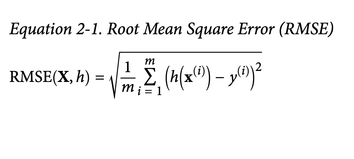
- What it’s ultimately trying to achieve: RMSE gives us a sense of how much error our system typically makes in its predictions, in the same units as the thing we’re predicting (dollars, in this case). It penalizes larger errors more heavily because of the squaring.
The book then introduces some common Notations (page 40), which are standard in ML:
m: Number of instances.x⁽ⁱ⁾: Feature vector for the i-th instance (all input attributes like longitude, population, etc., for one district).y⁽ⁱ⁾: Label for the i-th instance (the actual median house price for that district).X(capital X): Matrix containing all feature vectors for all instances (one row per district).h: The prediction function (our model), also called the hypothesis.ŷ⁽ⁱ⁾(y-hat): The predicted value for the i-th instance, i.e.,h(x⁽ⁱ⁾).
What if RMSE isn’t ideal? If you have many outliers, you might prefer Mean Absolute Error (MAE) (Equation 2-2, page 41).
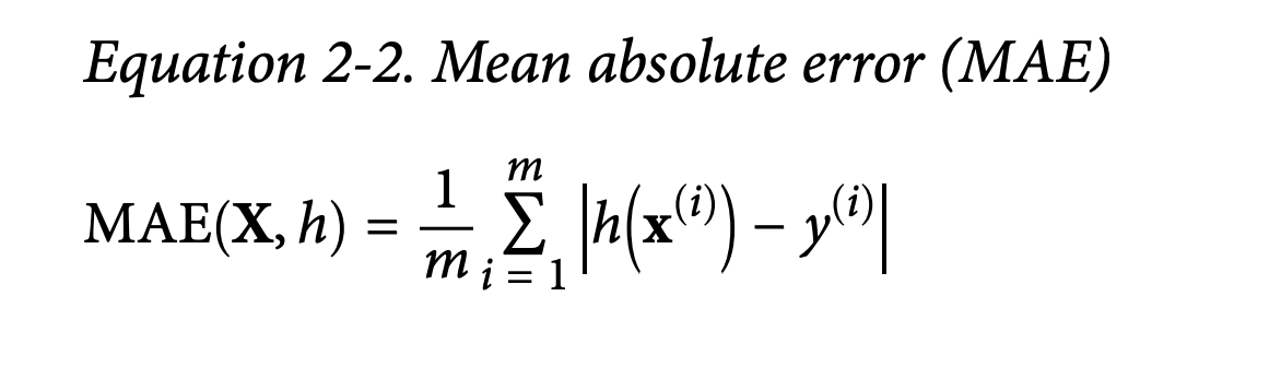
- What it’s trying to achieve: MAE measures the average absolute difference. It’s less sensitive to outliers than RMSE because it doesn’t square the errors.
The book connects these to different norms: RMSE is related to the Euclidean norm (l₂ norm – your standard straight-line distance), and MAE to the Manhattan norm (l₁ norm – like distance in a city grid). Generally, higher norm indices focus more on large values. RMSE (l₂) is usually preferred when outliers are rare (like in a bell-shaped distribution).(more details at the end of the chapter glossary)
Check the Assumptions (Page 42):
- Super important sanity check! We assume the downstream system needs actual price values. What if it actually converts prices into categories like “cheap,” “medium,” “expensive”? Then our regression task is overkill; it should have been a classification task!
- Fortunately, the book says our colleagues confirm they need actual prices. Phew!
(Page 42-50: Get the Data)
Time to get our hands dirty!
Create the Workspace (Page 42-45):
- This is about setting up your Python environment. The book walks through installing Python, Jupyter, NumPy, pandas, Matplotlib, and Scikit-Learn.
- It strongly recommends using an isolated environment (like
virtualenvorconda env). This is crucial in real projects to avoid library version conflicts. Think of it as a clean, dedicated lab space for each experiment. - Then, it shows how to start Jupyter and create a new notebook (Figure 2-3, 2-4).
Download the Data (Page 46):
- In real life, data might be in a database, spread across files, etc. Here, it’s simpler: a single compressed file.
- The book provides a nifty Python function
fetch_housing_data()to download and extract the data. Why a function? Automation! If data changes regularly, you can re-run the script.
Take a Quick Look at the Data Structure (Page 47-50):
- First, a function
load_housing_data()using pandas to load the CSV into a DataFrame. .head()(Figure 2-5): Shows the top 5 rows. We see attributes like longitude, latitude, housing_median_age, total_rooms, etc. 10 attributes in total..info()(Figure 2-6): Super useful!- 20,640 instances (rows) – fairly small for ML, but good for learning.
total_bedroomshas only 20,433 non-null values. This means 207 districts are missing this data. We’ll need to handle this!- Most attributes are
float64(numerical), butocean_proximityis anobject. Since it’s from a CSV, it’s likely text, probably categorical.
.value_counts()onocean_proximity(page 48) confirms it’s categorical:<1H OCEAN,INLAND, etc., with counts for each..describe()(Figure 2-7, page 49): Shows summary statistics for numerical attributes (count, mean, std, min, 25th/50th/75th percentiles, max).std(standard deviation) tells us how spread out the values are.- Percentiles (quartiles) give us a sense of the distribution. 25% of districts have
housing_median_age< 18.
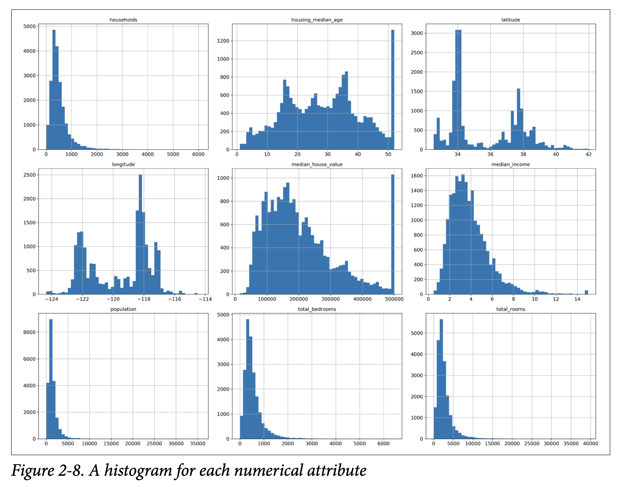
- Histograms (page 49, Figure 2-8 on page 50): A histogram for each numerical attribute.
This helps us see:
- Median Income: Doesn’t look like USD. The book clarifies it’s scaled (roughly tens of thousands of dollars) and capped at 15 (for high incomes) and 0.5 (for low incomes). Preprocessing is common.
- Housing Median Age & Median House Value: Also capped. The
median_house_valuecap (our target variable!) could be a problem. If the model learns prices never go above $500k, it can’t predict higher. We might need to get uncapped data or remove these districts. - Different Scales: Attributes have very different ranges (e.g.,
total_roomsvs.median_income). Many ML algorithms don’t like this. We’ll need feature scaling. - Tail-Heavy Distributions: Many histograms are skewed (e.g., extend far to the right). This can make it harder for algorithms to detect patterns. We might try transforming them (e.g., log transform) later.
- First, a function
(Page 51-55: Create a Test Set)
“Wait!” says the scorpion icon (page 51). “Before you look at the data any further, you need to create a test set, put it aside, and never look at it.”
- Why so early? Our brains are amazing pattern detectors. If we look too closely at the entire dataset, including what will be our test set, we might subconsciously pick up on patterns in the test data. This is data snooping bias. When we later evaluate our model on this “seen” test set, our performance estimate will be too optimistic. The model won’t generalize as well in the real world.
- How to create it? Theoretically, pick ~20% randomly and set aside.
- The book gives a simple
split_train_testfunction (page 52). - Problem: Running it again gives a different test set. Over time, your algorithm (or you!) might see the whole dataset.
- Solutions:
- Save the test set on the first run.
- Set a random seed (
np.random.seed(42)– 42 is the “Answer to the Ultimate Question of Life, the Universe, and Everything,” a common tongue-in-cheek seed).
- But these break if you fetch an updated dataset.
- Better solution for stable splits: Use a unique, immutable instance identifier. Compute a hash of the ID, and if the hash is below a threshold (e.g., 20% of max hash value), it goes into the test set. This ensures consistency even if the dataset is refreshed (new instances go to train/test consistently, old instances stay put).
- The housing dataset doesn’t have an ID column. Simplest is to use row index (if data is only ever appended). Or create an ID from stable features (e.g., latitude + longitude, though page 53 notes this can cause issues if coarse).
- The book gives a simple
- Scikit-Learn’s
train_test_split(page 53): Simpler, hasrandom_statefor reproducibility. Can also split multiple datasets (e.g., features and labels) consistently. - Stratified Sampling (Page 53-55):
- Random sampling is fine for large datasets. For smaller ones, you risk sampling bias. Imagine surveying 1000 people: random sampling might accidentally give you 60% men, not representative of the population.
- Stratified sampling ensures the test set is representative of important subgroups (strata).
- Experts say
median_incomeis very important. We want our test set to have a similar income distribution to the full dataset. - Since
median_incomeis continuous, we first create an income category attribute (pd.cut()) with 5 categories (Figure 2-9, page 54). Not too many strata, each large enough. - Then use Scikit-Learn’s
StratifiedShuffleSplitto sample, ensuring similar proportions of each income category in train and test sets. - Figure 2-10 (page 55) shows stratified sampling is much better than random sampling at preserving income category proportions.
- Finally, drop the temporary
income_catattribute. - This attention to test set creation is critical but often overlooked!
(Page 56-61: Discover and Visualize the Data to Gain Insights)
Now, working only with the training set (or a copy, strat_train_set.copy()):
Visualizing Geographical Data (Page 56-57):
- Scatter plot of
longitudevs.latitude(Figure 2-11). Looks like California, but hard to see patterns. - Setting
alpha=0.1(Figure 2-12) reveals high-density areas (Bay Area, LA, San Diego, Central Valley). - More advanced plot (Figure 2-13, page 57): Circle radius = population, color = median house price. Clearly shows prices are higher near coasts and in dense areas.
- Scatter plot of
Looking for Correlations (Page 58-60):
- Standard correlation coefficient (Pearson’s r): Ranges from -1 (strong negative correlation) to 1 (strong positive correlation). 0 means no linear correlation.
- Use
.corr()method on the DataFrame. corr_matrix["median_house_value"].sort_values(ascending=False)showsmedian_incomehas the strongest positive correlation (0.68) withmedian_house_value.- Figure 2-14 (page 59) shows examples: correlation only captures linear relationships. Nonlinear relationships can have r=0.
scatter_matrixfunction (pandas.plotting): Plots every numerical attribute against every other (Figure 2-15, page 60). Diagonal shows histograms. Focus on attributes promising for predictingmedian_house_value.- Zoom in on
median_incomevs.median_house_value(Figure 2-16, page 61):- Strong upward trend.
- Price cap at $500k clearly visible.
- Other less obvious horizontal lines (data quirks around $450k, $350k). Might want to remove these districts to prevent model learning these quirks.
Experimenting with Attribute Combinations (Page 61):
- Sometimes, combining attributes makes more sense.
total_roomsisn’t useful withouthouseholds. So, createrooms_per_household.- Similarly,
bedrooms_per_roomandpopulation_per_household. - Check correlations again (page 62).
bedrooms_per_roomis more negatively correlated with price thantotal_bedroomsortotal_rooms. Lower bedroom/room ratio (fewer bedrooms for a given house size, or larger rooms) often means more expensive.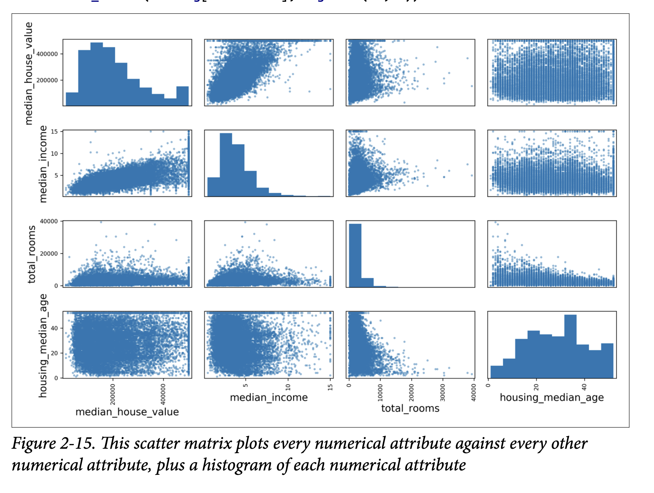
This exploration is iterative. Get a prototype, analyze its output, come back here.
(Page 62-71: Prepare the Data for Machine Learning Algorithms)
Time to write functions for data transformations. Why functions?
- Reproducibility.
- Build a library of transformations.
- Use in live system for new data.
First, revert to a clean training set and separate predictors (housing) from labels (housing_labels).
Data Cleaning (Missing Values - page 63):
- We saw
total_bedroomshas missing values. Options:- Get rid of corresponding districts:
housing.dropna(subset=["total_bedrooms"]) - Get rid of the whole attribute:
housing.drop("total_bedrooms", axis=1) - Set values to something (zero, mean, median):
median = housing["total_bedrooms"].median(), thenhousing["total_bedrooms"].fillna(median, inplace=True)
- Get rid of corresponding districts:
- If using option 3, compute median on training set and save it to fill missing values in test set and live data.
- Scikit-Learn’s
SimpleImputer(page 63):- Create an imputer:
imputer = SimpleImputer(strategy="median") - It only works on numerical attributes, so drop
ocean_proximityfirst:housing_num = housing.drop("ocean_proximity", axis=1) - Fit the imputer to numerical training data:
imputer.fit(housing_num)(computes medians). - The medians are stored in
imputer.statistics_. - Transform the training set:
X = imputer.transform(housing_num)(returns NumPy array). - Convert back to DataFrame if needed.
- Create an imputer:
- Scikit-Learn Design Principles (sidebar, page 64-65):
- Consistency: Estimators, Transformers, Predictors.
- Estimators: Any object that can estimate params from data (e.g.,
imputer).fit(data, [labels])method. Hyperparameters set in constructor. - Transformers: Estimators that can transform data (e.g.,
imputer).transform(data)method. Alsofit_transform()(often optimized). - Predictors: Estimators that can make predictions (e.g.,
LinearRegression).predict(data)method.score(data, labels)method. - Inspection: Hyperparameters are public instance vars (e.g.,
imputer.strategy). Learned params end with_(e.g.,imputer.statistics_). - Nonproliferation of classes: Uses NumPy arrays, basic Python types.
- Composition: Easy to combine (e.g.,
Pipeline). - Sensible defaults.
- We saw
Handling Text and Categorical Attributes (Page 65-67):
ocean_proximityis categorical.OrdinalEncoder(Scikit-Learn >= 0.20): Converts categories to numbers (0, 1, 2…). (Page 66).- Problem: ML algorithms assume nearby numbers are more similar (e.g., 0 and 1 more similar than 0 and 4). This isn’t true for
ocean_proximity.
- Problem: ML algorithms assume nearby numbers are more similar (e.g., 0 and 1 more similar than 0 and 4). This isn’t true for
OneHotEncoder(Scikit-Learn): Common solution (page 67). Creates one binary attribute per category (dummy variables). Only one is “hot” (1), others “cold” (0).- Output is a SciPy sparse matrix (efficient for many categories, as it only stores non-zero locations). Can convert to dense with
.toarray().
- Output is a SciPy sparse matrix (efficient for many categories, as it only stores non-zero locations). Can convert to dense with
- If many categories, one-hot encoding creates many features. Alternatives: replace with numerical related features (e.g., distance to ocean) or use embeddings (learnable low-dimensional vectors, Ch 13 & 17).
Custom Transformers (Page 68):
- For custom cleanup or attribute combination.
- Create a class, implement
fit(),transform(),fit_transform(). - Add
TransformerMixin(getsfit_transform()for free) andBaseEstimator(getsget_params(),set_params()for hyperparameter tuning, if no*args,**kwargsin constructor). - Example:
CombinedAttributesAdderclass to addrooms_per_householdetc. Has a hyperparameteradd_bedrooms_per_room.
Feature Scaling (Page 69):
- Crucial! ML algos often perform badly if numerical inputs have very different scales.
- Two common ways:
- Min-max scaling (Normalization): Values shifted/rescaled to range 0-1. Subtract min, divide by (max-min). Scikit-Learn:
MinMaxScaler. - Standardization: Subtract mean, divide by std dev. Resulting distribution has zero mean, unit variance. Not bounded to a specific range. Less affected by outliers. Scikit-Learn:
StandardScaler.
- Min-max scaling (Normalization): Values shifted/rescaled to range 0-1. Subtract min, divide by (max-min). Scikit-Learn:
- Important: Fit scalers on training data only! Then use them to transform train set, test set, and new data.
Transformation Pipelines (Page 70-71):
- Many data prep steps need to be in order. Scikit-Learn’s
Pipelinehelps. - Example
num_pipelinefor numerical attributes (page 70):SimpleImputer->CombinedAttributesAdder->StandardScaler. - Call
pipeline.fit_transform(housing_num). ColumnTransformer(Scikit-Learn >= 0.20): Applies different transformers to different columns. Super convenient! (Page 71)- Takes list of (name, transformer, column_list) tuples.
- Applies
num_pipelineto numerical columns,OneHotEncoderto categorical. - Concatenates outputs. Handles sparse/dense matrix mix.
- This gives one preprocessing pipeline for all data!
- Many data prep steps need to be in order. Scikit-Learn’s
(Page 72-74: Select and Train a Model)
Finally, the exciting part!
Training and Evaluating on the Training Set (Page 72):
- Linear Regression:
lin_reg = LinearRegression()lin_reg.fit(housing_prepared, housing_labels)- Try on a few instances: predictions aren’t great.
- RMSE on whole training set: $68,628. Not good (most house values are $120k-$265k). This is underfitting. Features might not be good enough, or model too simple.
- Decision Tree Regressor (more complex model, Ch 6):
tree_reg = DecisionTreeRegressor()tree_reg.fit(housing_prepared, housing_labels)- Evaluate on training set: RMSE = 0.0! Perfect? (Page 73)
- No, much more likely it badly overfit the data.
- Don’t touch test set yet! Use part of training set for validation.
- Linear Regression:
Better Evaluation Using Cross-Validation (Page 73-74):
- Option 1:
train_test_splittraining set into smaller train/validation. - Option 2 (better): K-fold cross-validation.
- Scikit-Learn’s
cross_val_score. Splits training set into K folds (e.g., 10). Trains K times, each time using a different fold for evaluation and other K-1 folds for training. Returns K scores. - Scoring function:
cross_val_scoreexpects utility (higher is better), not cost (lower is better). So usescoring="neg_mean_squared_error". Then takenp.sqrt(-scores). - Decision Tree CV scores (page 74): Mean RMSE ~71,407. Standard deviation ~2,439. Much worse than 0! And worse than Linear Regression.
- Linear Regression CV scores: Mean RMSE ~69,052. Std dev ~2,732.
- Decision Tree is overfitting badly.
- Scikit-Learn’s
- Random Forest Regressor (Ensemble Learning, Ch 7):
- Trains many Decision Trees on random subsets of features, averages predictions.
- Skip code details (similar to others).
- Training set RMSE (page 75,
forest_rmse): ~18,603. - CV scores: Mean RMSE ~50,182. Std dev ~2,097.
- Much better! But training score is still much lower than validation scores -> still overfitting. Solutions: simplify model, regularize, get more data.
- Goal: Shortlist 2-5 promising models (SVMs, neural nets, etc.) without too much hyperparameter tweaking yet.
- Save your models! Use
joblib(better for large NumPy arrays) orpickle. Save hyperparameters, CV scores, predictions.
- Option 1:
(Page 75-78: Fine-Tune Your Model)
Now, take your shortlisted models and fine-tune their hyperparameters.
Grid Search (Page 76):
- Tedious to do manually. Use Scikit-Learn’s
GridSearchCV. - Tell it which hyperparameters to try and what values.
- It uses cross-validation to evaluate all combinations.
- Example
param_gridforRandomForestRegressor. - It will explore (3x4 + 2x3) = 18 combinations, each trained 5 times (for cv=5). 90 rounds of training!
grid_search.best_params_gives the best combination.grid_search.best_estimator_gives the best model retrained on the full training set (ifrefit=True, default).- Evaluation scores for each combo are in
grid_search.cv_results_. - Example result (page 77): RMSE 49,682. Better than default 50,182.
- Can treat data prep steps as hyperparameters too! (e.g.,
add_bedrooms_per_roomin your custom transformer).
- Tedious to do manually. Use Scikit-Learn’s
Randomized Search (Page 78):
RandomizedSearchCV. Good for large hyperparameter search spaces.- Instead of trying all combos, evaluates a given number of random combinations.
- Benefits: explores more values per hyperparameter if run long enough; more control over budget.
Ensemble Methods (Page 78):
- Combine best models. Often performs better than any single model, especially if they make different types of errors. (More in Ch 7).
Analyze the Best Models and Their Errors (Page 78-79):
- Gain insights!
RandomForestRegressorcan show feature importances. - List importances with attribute names (page 79).
median_incomeis most important.INLAND(categorical feature) is surprisingly important. - Might decide to drop less useful features.
- Look at specific errors your system makes. Why? How to fix?
- Gain insights!
(Page 79-80: Evaluate Your System on the Test Set)
The moment of truth! After all tweaking, evaluate the final model on the test set.
- Get predictors (
X_test) and labels (y_test) fromstrat_test_set. - Run
full_pipeline.transform(X_test)(NOTfit_transform– don’t fit to test set!). final_model = grid_search.best_estimator_final_predictions = final_model.predict(X_test_prepared)final_mse = mean_squared_error(y_test, final_predictions)final_rmse = np.sqrt(final_mse)-> e.g., 47,730.- Point estimate might not be enough. Compute a 95% confidence interval using
scipy.stats.t.interval(). - If performance is worse than CV scores (often is due to tuning on validation set), resist temptation to tweak based on test set results! Those tweaks are unlikely to generalize.
(Page 80-83: Launch, Monitor, and Maintain Your System)
You got approval to launch!
- Prelaunch: Present solution, highlight learnings, assumptions, limitations. Document. Create clear visualizations.
- Launch: Polish code, write docs, tests. Deploy model.
- Save trained pipeline (e.g., with
joblib). - Load in production environment.
- Maybe wrap in a web service that your app queries via REST API (Figure 2-17, page 81). Easier upgrades, scaling.
- Or deploy on cloud (e.g., Google Cloud AI Platform).
- Save trained pipeline (e.g., with
- Monitor: This is not the end!
- Check live performance regularly. Trigger alerts if it drops.
- Models “rot” over time as the world changes. (Cats and dogs don’t mutate, but camera tech and breed popularity do!)
- Infer performance from downstream metrics (e.g., sales of recommended products).
- Or use human raters / crowdsourcing (Amazon Mechanical Turk) for tasks needing human judgment.
- Monitor input data quality (malfunctioning sensors, stale data from other teams).
- Maintain:
- Automate as much as possible:
- Collect fresh data regularly and label it.
- Script to retrain model and fine-tune hyperparameters.
- Script to evaluate new vs. old model on updated test set, deploy if better.
- Keep backups of models and datasets. Easy rollback. Compare new models to old.
- Evaluate on specific subsets of test data for deeper insights (e.g., recent data, specific input types like inland vs. ocean districts).
- Automate as much as possible:
ML involves a lot of infrastructure! First project is a lot of effort. Once it’s in place, future projects are faster.
(Page 83-84: Try It Out! & Exercises) The chapter ends by encouraging you to try this whole process on a dataset you’re interested in (e.g., from Kaggle). And then lists some great exercises based on the housing dataset. Definitely try these!
Glossary
RMSE , MAE a Deep dive
Think about it this way: both RMSE (Root Mean Square Error) and MAE (Mean Absolute Error) are trying to tell us, on average, how “far off” our model’s predictions are from the actual values. The “how far off” part is where the idea of “distance” comes in, and norms are just formal mathematical ways of defining distance.
Let’s look at a single prediction error first. Suppose the actual house price (y) is $300,000 and our model predicts (ŷ) $250,000. The error is $50,000.
MAE (Mean Absolute Error) and the l₁ norm (Manhattan Distance):
- MAE takes the absolute value of this error: |$250,000 - $300,000| = $50,000.
- Then it averages these absolute errors over all your predictions.
- The l₁ norm (read as “L-one norm”) of a vector (think of a vector of errors
[e₁, e₂, ..., eₘ]) is the sum of the absolute values of its components:|e₁| + |e₂| + ... + |eₘ|. The MAE is just this sum divided bym(the number of errors). - Why “Manhattan Distance”? Imagine you’re in a city like Manhattan where streets form a grid. To get from point A to point B, you can’t cut diagonally through buildings. You have to travel along the streets (say, 3 blocks east and 4 blocks north). The total distance is 3 + 4 = 7 blocks. This is the l₁ distance. You’re summing the absolute differences along each axis (the “east-west” error and the “north-south” error, if you will). In our error context, we only have one “axis” of error for each prediction, and MAE sums these absolute “street-block” errors.
RMSE (Root Mean Square Error) and the l₂ norm (Euclidean Distance):
- RMSE takes the error ($50,000), squares it (($50,000)² = 2,500,000,000), then averages these squared errors, and finally takes the square root of that average.
- The l₂ norm (read as “L-two norm”) of a vector of errors
[e₁, e₂, ..., eₘ]is√(e₁² + e₂² + ... + eₘ²). - Why “Euclidean Distance”? This is the “as the crow flies” distance you learned in geometry using the Pythagorean theorem:
distance = √(Δx² + Δy²). If you have a vector of errors, the l₂ norm is like calculating the length of that vector in a multi-dimensional space. It’s our everyday understanding of straight-line distance. - When RMSE squares the errors, it gives much more weight to larger errors. An error of 10 becomes 100, but an error of 2 becomes 4. The error of 10 contributes 25 times more to the sum of squares than the error of 2 (100 vs 4), whereas for MAE, it would only contribute 5 times more (10 vs 2). The square root at the end brings the measurement back into the original units (e.g., dollars).
So, what’s the ultimate goal of connecting them to norms?
Generalization: Norms are a general mathematical concept for measuring the “size” or “length” of vectors. By recognizing that RMSE and MAE are related to specific norms (l₂ and l₁ respectively), it places them within a broader mathematical framework. There are other norms too (l₀, l∞, lₚ in general), and each has different properties and might be useful in different contexts for measuring error or regularizing models.
- For instance, the l₀ norm counts the number of non-zero elements in a vector.
- The l∞ (L-infinity) norm gives the maximum absolute value in a vector (it focuses only on the largest error).
Understanding Properties: Knowing the underlying norm helps us understand the properties of the error metric.
- Because RMSE uses the l₂ norm (squaring), it’s more sensitive to outliers. One very large error, when squared, can dominate the RMSE.
- Because MAE uses the l₁ norm (absolute value), it’s more robust to outliers. A large error is just a large error; it’s not disproportionately magnified.
Consistency in Terminology: In more advanced ML literature, you’ll often see error functions or regularization terms described using norm notation (e.g., “l₁ regularization” or “l₂ regularization”). Understanding this connection early on helps you navigate that.
Let’s try a simple analogy:
Imagine you have two friends, Alex (l₁) and Beth (l₂), and you ask them to measure how “messy” a room is based on how far items are from their correct places.
- Alex (l₁ / MAE): For each misplaced item, Alex measures how far it is from its spot (e.g., book is 2 feet off, sock is 3 feet off). Alex just adds up these distances (2+3=5 feet of “mess”). Alex treats every foot of displacement equally.
- Beth (l₂ / RMSE): For each misplaced item, Beth measures the distance, squares it (book 2²=4, sock 3²=9), adds them up (4+9=13), and then might take a square root. Beth gets really upset by items that are very far off, because squaring makes those large distances much bigger. A sock 10 feet away (10²=100) is much, much worse to Beth than 5 socks each 2 feet away (5 * 2² = 20).
So, when the book says “RMSE corresponds to the Euclidean norm” and “MAE corresponds to the l₁ norm,” it’s essentially saying:
- RMSE measures error in a way that emphasizes large errors more (like a straight-line distance calculation that involves squaring).
- MAE measures error in a way that treats all magnitudes of error more evenly (like adding up block-by-block distances).
Did that make it a bit clearer? The key is that they are both ways to quantify “how far off” you are, but they “feel” or “react” to large errors differently because of their mathematical structure, which is captured by these different types of norms.