Chapter 4: Training Models
53 min readChapter 4: Training Models.
Introduction - Beyond Black Boxes
Up until now, as the book says, we’ve treated ML models and their training algorithms mostly like black boxes. We fed them data, they gave us results, and we learned to evaluate those results. You’ve optimized regression, improved classifiers, even built a spam filter, often without peeking under the hood. And that’s okay for many practical purposes!
However, understanding how these things work internally is incredibly powerful. It helps you:
- Choose the right model and algorithm: Knowing the mechanics helps you match the tool to the task.
- Select good hyper parameters: Hyper parameters often control the learning process itself. Understanding that process helps you tune them effectively.
- Debug issues and perform error analysis: When things go wrong, or your model makes weird mistakes, knowing the “why” is crucial.
- Foundation for advanced topics: Especially for neural networks (Part II of the book), the concepts here are fundamental.
This chapter focuses on Linear Regression as a starting point because it’s simple, yet we can train it in very different ways. We’ll explore two main approaches:
- A direct “closed-form” equation (The Normal Equation): This is like having a magic formula that directly spits out the best model parameters in one go.
- An iterative optimization approach (Gradient Descent): This is more like a trial-and-error process. We start with a guess for the parameters and gradually tweak them, step by step, to minimize the error, eventually (hopefully!) arriving at the same best parameters. We’ll see different “flavors” of Gradient Descent: Batch, Mini-batch, and Stochastic.
Then, the chapter will touch on:
- Polynomial Regression: How to use linear models for non-linear data.
- Learning Curves: Tools to diagnose over fitting or under fitting.
- Regularization: Techniques to prevent over fitting.
- Logistic Regression and Softmax Regression: Models commonly used for classification tasks.
The scorpion icon on page 112 gives a fair warning: there will be some math (linear algebra, calculus). If you’re “allergic,” the book suggests you can still get the concepts by focusing on the text. My job is to make sure you get those concepts, regardless of how comfortable you are with the equations. We’ll always ask: “What is this equation ultimately trying to achieve?”
Linear Regression - The Model
Remember our life satisfaction model from Chapter 1? life_satisfaction = θ₀ + θ₁ × GDP_per_capita. That was a simple linear regression with one feature.
More generally, a linear model predicts a value by:
- Taking all the input features (like a house’s square footage, number of bedrooms, age, etc.).
- Multiplying each feature by a specific weight (a model parameter).
- Summing up these weighted features.
- Adding a constant bias term (another model parameter, also called the intercept).
Equation 4-1 (page 112): Linear Regression model prediction
ŷ = θ₀ + θ₁x₁ + θ₂x₂ + ⋯ + θₙxₙ
ŷ(y-hat): The predicted value.n: The number of features.xᵢ: The value of the i-th feature.θ₀: The bias term (theta-zero). What it’s ultimately trying to achieve: It’s the baseline prediction if all feature values were zero. It allows the line/plane to shift up or down.θ₁toθₙ: The feature weights.θⱼis the weight for the j-th feature. What they’re ultimately trying to achieve: They represent how much a one-unit change in that featurexⱼaffects the predicted valueŷ, holding other features constant. A positive weight means the feature positively influences the prediction; a negative weight means it negatively influences it. The magnitude shows the strength of the influence.
Equation 4-2 (page 113): Vectorized form
ŷ = h_θ(x) = θ · x
This is just a more compact way to write Equation 4-1 using vector notation.
θ(theta): Is now a parameter vector[θ₀, θ₁, ..., θₙ].x: Is the instance’s feature vector[x₀, x₁, ..., xₙ]. Here, we add a “dummy” featurex₀which is always set to 1. This allows us to include the bias termθ₀neatly into the dot product (becauseθ₀ * x₀ = θ₀ * 1 = θ₀).θ · x: This is the dot product of the two vectors. It’s exactly the sumθ₀x₀ + θ₁x₁ + ... + θₙxₙ.h_θ(x): This is our hypothesis function (our model), parameterized byθ. Given an inputx, it predictsŷ.
The bird sidebar (page 113) explains that vectors are often column vectors (2D arrays with one column). So, if θ and x are column vectors, the dot product can be written as a matrix multiplication: ŷ = θᵀx (where θᵀ is the transpose of θ, making it a row vector). Don’t let this bog you down; it’s a notational convenience. The goal is the same: calculate a weighted sum of features plus a bias.
How do we train it?
Training means finding the values for the parameters θ (the bias θ₀ and the weights θ₁ to θₙ) that make the model “best fit” the training data.
To do this, we need a way to measure how well (or poorly) the model fits. We learned in Chapter 2 that for regression, a common measure is RMSE (Root Mean Square Error).
- What it’s ultimately trying to achieve: Quantify the typical prediction error. However, for mathematical convenience during training, it’s often easier to minimize the MSE (Mean Squared Error) instead. Minimizing MSE will also minimize RMSE (since the square root function is monotonic). The footnote on page 113 is important: the function we optimize during training (the cost function, here MSE) might be different from the final performance metric we use to evaluate the model (e.g., RMSE). This is often because the cost function has nice mathematical properties (like being easily differentiable) that make optimization easier.
MSE Cost Function & The Normal Equation
Equation 4-3 (page 114): MSE cost function for a Linear Regression model
MSE(X, h_θ) = (1/m) * Σᵢ (θᵀx⁽ⁱ⁾ - y⁽ⁱ⁾)²
(summing from i=1 to m, where m is the number of instances)
- What it’s ultimately trying to achieve:
- For each training instance
i:θᵀx⁽ⁱ⁾is the model’s prediction for that instance.y⁽ⁱ⁾is the actual target value.(θᵀx⁽ⁱ⁾ - y⁽ⁱ⁾)is the error for that instance.- We square this error:
(error)². (Why square? It makes all errors positive, and it penalizes larger errors more heavily).
- We sum these squared errors over all
mtraining instances:Σᵢ (error)². - We divide by
mto get the mean of the squared errors. This function tells us, on average, how “bad” our model’s predictions are for a given set of parametersθ. Our goal in training is to find theθthat makes this MSE as small as possible.
- For each training instance
The Normal Equation: A Direct Solution
For Linear Regression with an MSE cost function, there’s a wonderful mathematical shortcut. Instead of iteratively searching for the best θ, there’s a direct formula that gives you the θ that minimizes the cost function in one shot! This is called the Normal Equation.
Equation 4-4 (page 114): Normal Equation
θ̂ = (XᵀX)⁻¹ Xᵀy
θ̂(theta-hat): This is the value ofθthat minimizes the cost function.X: The matrix of input features for all training instances (each row is an instance,x₀for each instance is 1).y: The vector of actual target values for all training instances.Xᵀ: The transpose of matrixX.(XᵀX)⁻¹: The inverse of the matrixXᵀX.
What it’s ultimately trying to achieve: This equation, derived using calculus (setting the derivative of the cost function to zero and solving for θ), directly calculates the optimal parameter vector θ̂ that makes the linear model fit the training data as closely as possible (in the mean squared error sense). It’s like a direct recipe: plug in your data X and y, and out pops the best θ.
Testing the Normal Equation
The book generates some linear-looking data (Figure 4-1):
X = 2 * np.random.rand(100, 1) (100 instances, 1 feature)
y = 4 + 3 * X + np.random.randn(100, 1) (True model is y = 4 + 3x₁ + noise)
So, the ideal θ₀ is 4, and the ideal θ₁ is 3.
To use the Normal Equation, we need to add x₀ = 1 to each instance in X:
X_b = np.c_[np.ones((100, 1)), X] (np.c_ concatenates arrays column-wise)
Now, apply the Normal Equation:
theta_best = np.linalg.inv(X_b.T.dot(X_b)).dot(X_b.T).dot(y)
The result is something like [[4.215...], [2.770...]].
So, θ₀̂ ≈ 4.215 and θ₁̂ ≈ 2.770.
It’s close to the true values (4 and 3), but not exact because of the random noise we added to y. The noise makes it impossible to recover the exact original parameters.
We can then use this theta_best to make predictions (Figure 4-2).
Scikit-Learn and Computational Complexity
Scikit-Learn
LinearRegression:from sklearn.linear_model import LinearRegressionlin_reg = LinearRegression()lin_reg.fit(X, y)Scikit-Learn handles adding thex₀=1feature (or rather, it separates the bias termlin_reg.intercept_from the feature weightslin_reg.coef_). The results are the same as the Normal Equation.Underlying Method (
scipy.linalg.lstsq): Scikit-Learn’sLinearRegressionactually usesscipy.linalg.lstsq()(“least squares”). This function computesθ̂ = X⁺y, whereX⁺is the pseudoinverse (or Moore-Penrose inverse) ofX. You can computeX⁺usingnp.linalg.pinv(). The pseudoinverse is calculated using a technique called Singular Value Decomposition (SVD).- Why SVD/pseudoinverse instead of the direct Normal Equation
(XᵀX)⁻¹ Xᵀy?- More efficient: SVD is generally more computationally efficient.
- Handles edge cases: The Normal Equation requires
XᵀXto be invertible. If it’s not (e.g., if you have more features than instances,m < n, or if some features are redundant/linearly dependent), the Normal Equation breaks down. The pseudoinverse is always defined, making SVD more robust.
- Why SVD/pseudoinverse instead of the direct Normal Equation
Computational Complexity:
- Normal Equation (inverting
XᵀX): About O(n²·⁴) to O(n³) wherenis the number of features. This gets very slow if you have many features (e.g., 100,000 features). Doubling features can increase time by 5-8x. - SVD (used by Scikit-Learn): About O(n²). Doubling features increases time by ~4x. Still slow for very large
n. - Both are O(m) with respect to the number of instances
m. So, they handle large numbers of training instances efficiently, as long as the data fits in memory. - Predictions: Once trained, making predictions is very fast: O(m) and O(n) – linear with number of instances and features.
- Normal Equation (inverting
The Problem with Normal Equation/SVD: They get slow with many features and require all data to be in memory. This leads us to the next method…
Gradient Descent - The Iterative Approach
When the Normal Equation is too slow (too many features) or the dataset is too large to fit in memory, we need a different approach. Enter Gradient Descent.
The Core Idea: Gradient Descent is a generic optimization algorithm. It iteratively tweaks model parameters to minimize a cost function.
- Imagine you’re lost in a foggy mountain valley. You can only feel the slope of the ground under your feet. To get to the bottom, you’d take a step in the direction of the steepest downhill slope. Repeat.
- This is Gradient Descent:
- It measures the local gradient of the cost function (e.g., MSE) with respect to the parameter vector
θ. The gradient tells you the direction of steepest ascent. - It takes a step in the opposite direction (descending gradient) to reduce the cost.
- Repeat until the gradient is zero (or very close), meaning you’ve reached a minimum.
- It measures the local gradient of the cost function (e.g., MSE) with respect to the parameter vector
The Process (Figure 4-3, page 118):
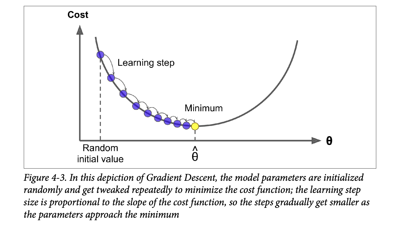
- Random Initialization: Start with random values for
θ. - Iterative Improvement: In each step:
- Calculate the gradient of the cost function at the current
θ. - Update
θby taking a small step in the negative gradient direction.
- Calculate the gradient of the cost function at the current
- Convergence: Continue until the algorithm converges to a minimum (cost stops decreasing significantly).
- Random Initialization: Start with random values for
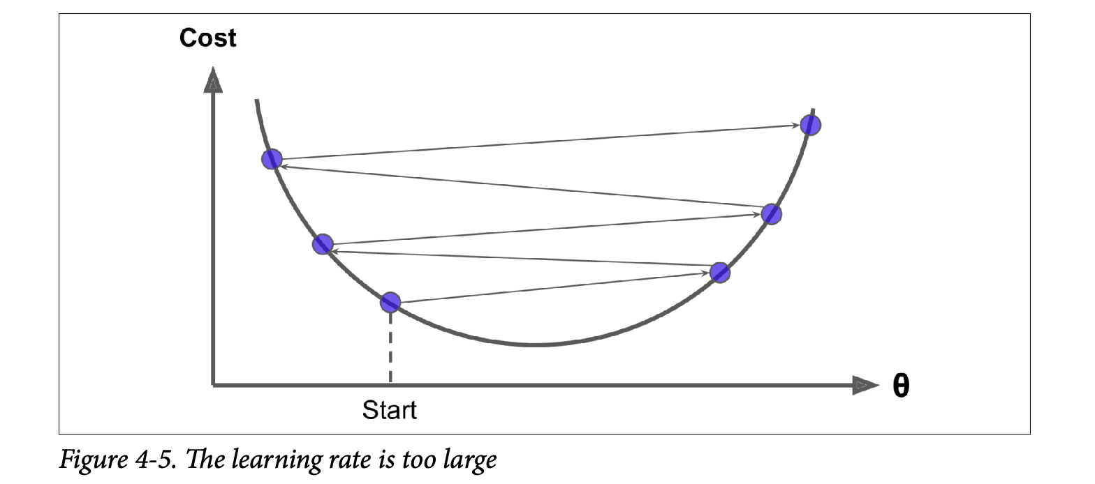
Learning Rate (η - eta):
- This is a crucial hyperparameter that determines the size of the steps.
- Too small (Figure 4-4): Many iterations needed to converge (very slow).
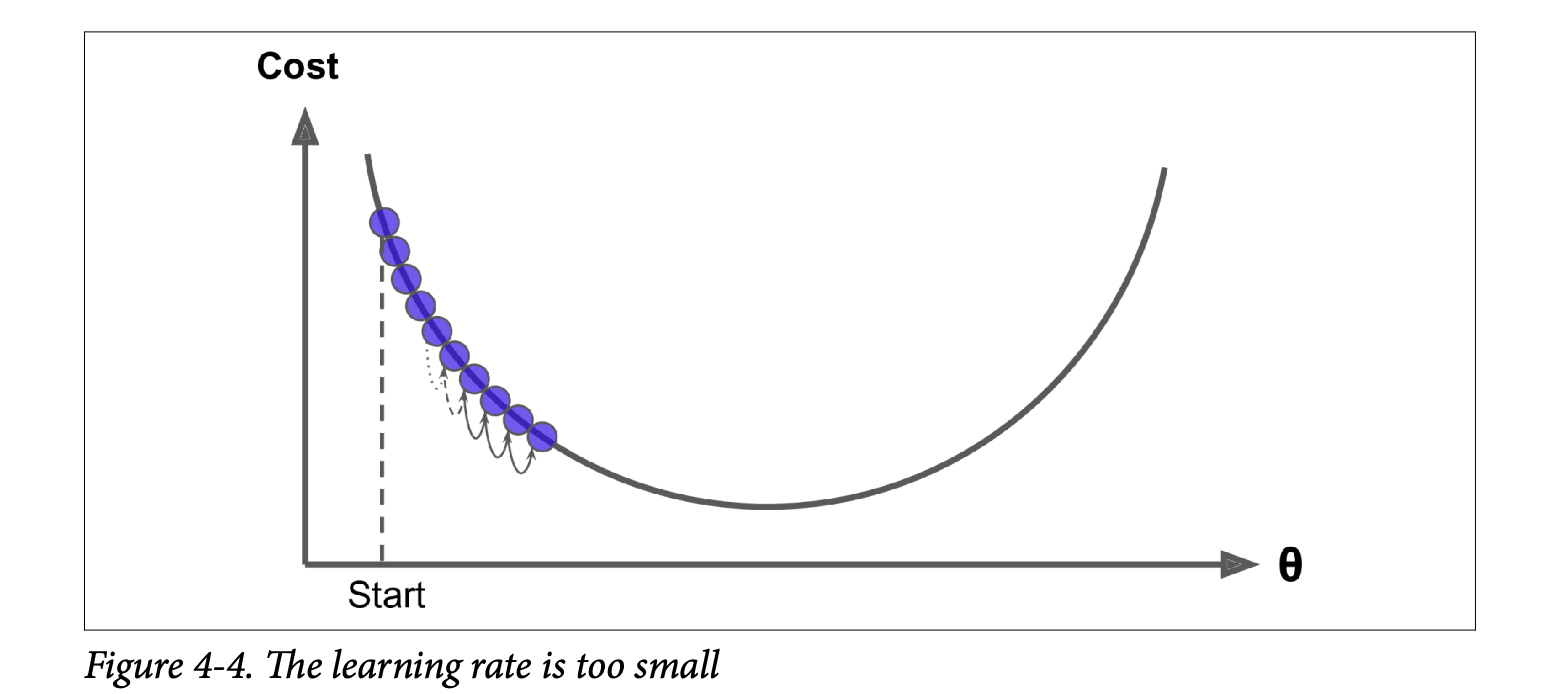
- Too large (Figure 4-5): Might jump across the valley, diverge, and fail to find a solution.
Challenges (Figure 4-6, page 119):
- Local Minima: If the cost function has multiple minima (not a smooth bowl), GD might converge to a local minimum, which isn’t as good as the global minimum.
- Plateaus: If the cost function has flat areas, GD can take a very long time to cross them.
- Irregular Terrains: Holes, ridges make convergence difficult.
Good News for Linear Regression MSE:
- The MSE cost function for Linear Regression is a convex function.
- What this means: It’s shaped like a bowl. It has no local minima, only one global minimum.
- It’s also continuous with a slope that doesn’t change abruptly.
- Consequence: Gradient Descent is guaranteed to approach the global minimum if you wait long enough and the learning rate isn’t too high.
- The MSE cost function for Linear Regression is a convex function.
Feature Scaling Matters! (Figure 4-7, page 120):
- If features have very different scales (e.g., feature 1 ranges 0-1, feature 2 ranges 0-1000), the cost function “bowl” becomes elongated.
- GD will take a long, zig-zag path to the minimum.
- Solution: Ensure all features have a similar scale (e.g., using
StandardScaler). GD will then converge much faster.
Parameter Space: Training a model is essentially a search in the model’s parameter space for the combination of parameters that minimizes the cost. More parameters = higher dimensional space = harder search. For Linear Regression (convex cost), it’s like finding the bottom of a D-dimensional bowl.
Batch Gradient Descent - BGD
To implement GD, we need the gradient of the cost function with respect to each model parameter θⱼ. This is the partial derivative ∂MSE(θ) / ∂θⱼ.
Equation 4-5 (page 121): Partial derivative of MSE w.r.t.
θⱼ∂MSE(θ)/∂θⱼ = (2/m) * Σᵢ (θᵀx⁽ⁱ⁾ - y⁽ⁱ⁾) * xⱼ⁽ⁱ⁾- What it’s ultimately trying to achieve: For each parameter
θⱼ, it calculates how much the MSE would change ifθⱼchanged a tiny bit.(θᵀx⁽ⁱ⁾ - y⁽ⁱ⁾)is the prediction error for instancei.- We multiply this error by the value of the
j-th feature of instancei,xⱼ⁽ⁱ⁾. (Ifxⱼ⁽ⁱ⁾is large,θⱼhas a bigger impact on the prediction and thus on the error). - We average this product over all instances
m.
- What it’s ultimately trying to achieve: For each parameter
Equation 4-6 (page 122): Gradient vector
∇_θ MSE(θ)∇_θ MSE(θ) = (2/m) Xᵀ(Xθ - y)- This is the compact, vectorized way to compute all partial derivatives at once.
∇_θ MSE(θ)is a vector containing∂MSE(θ)/∂θ₀,∂MSE(θ)/∂θ₁, …,∂MSE(θ)/∂θₙ. - What it’s ultimately trying to achieve: It gives the direction of steepest increase in the cost function.
Crucial point for BATCH GD: This formula uses the entire training set
Xat each step to calculate the gradients. This is why it’s called Batch Gradient Descent.- Consequence: Terribly slow on very large training sets.
- Advantage: Scales well with the number of features (unlike Normal Equation).
- This is the compact, vectorized way to compute all partial derivatives at once.
Equation 4-7 (page 122): Gradient Descent step
θ⁽ⁿᵉˣᵗ ˢᵗᵉᵖ⁾ = θ - η ∇_θ MSE(θ)- What it’s ultimately trying to achieve: Update the current parameters
θby taking a step of sizeη(learning rate) in the direction opposite to the gradient (downhill).
- What it’s ultimately trying to achieve: Update the current parameters
Implementation (page 122): The code shows a loop:
for iteration in range(n_iterations):gradients = 2/m * X_b.T.dot(X_b.dot(theta) - y)theta = theta - eta * gradientsWitheta = 0.1andn_iterations = 1000, the resultingthetais exactly what the Normal Equation found! Perfect.Effect of Learning Rate
η(Figure 4-8, page 123):η = 0.02(left): Too slow, many steps to converge.η = 0.1(middle): Good, converges quickly.η = 0.5(right): Too high, diverges, jumps around.
Finding a good learning rate: Grid search (Chapter 2).
Setting number of iterations: If too low, far from optimum. If too high, waste time after convergence.
- Solution: Set many iterations, but stop when the gradient vector becomes tiny (its norm <
ϵ, a small tolerance). This means we’re (almost) at the minimum.
- Solution: Set many iterations, but stop when the gradient vector becomes tiny (its norm <
Convergence Rate (sidebar, page 124): For convex cost functions like MSE, BGD with fixed
ηtakes O(1/ϵ) iterations to reach withinϵof the optimum. To get 10x more precision (divideϵby 10), you need ~10x more iterations.
Stochastic Gradient Descent - SGD
Batch GD is slow on large datasets because it uses all training data at each step.
Stochastic Gradient Descent (SGD):
- At each step, picks one random instance from the training set and computes gradients based only on that single instance.
- Advantages:
- Much faster per step (very little data to process).
- Can train on huge datasets (only one instance in memory at a time – good for out-of-core learning, Ch 1).
- Disadvantages (Figure 4-9, page 124):
- Stochastic nature: The path to the minimum is much more erratic (“bouncy”) than BGD. Cost function goes up and down, decreasing only on average.
- Never settles: Once near the minimum, it keeps bouncing around, never perfectly settling. Final parameters are good, but not optimal.
- Advantage of randomness: If cost function is irregular (non-convex, Figure 4-6), SGD’s randomness can help it jump out of local minima and find a better global minimum.
Learning Schedule (page 125):
- To help SGD settle at the minimum, we can gradually reduce the learning rate
η. - Start with large
η(quick progress, escape local minima). - Make
ηsmaller over time (settle at global minimum). - This is like simulated annealing in metallurgy.
- The function determining
ηat each iteration is the learning schedule. - If
ηreduces too quickly -> stuck in local minimum or frozen half-way. - If
ηreduces too slowly -> bounce around minimum for long, or stop too early with suboptimal solution.
- To help SGD settle at the minimum, we can gradually reduce the learning rate
Implementation of SGD (page 125):
- Outer loop for
epochs(an epoch is one pass through the entire training set, by convention). - Inner loop for
miterations (number of instances). In each inner iteration:- Pick a
random_index. - Get
xiandyifor that instance. - Gradients calculated using only
xiandyi:gradients = 2 * xi.T.dot(xi.dot(theta) - yi). (Note:2not2/mbecausem=1here). - Update
etausinglearning_schedule(epoch * m + i). - Update
theta.
- Pick a
- After 50 epochs (much fewer iterations than BGD’s 1000), it finds a
thetavery close to BGD’s. - Figure 4-10 (page 126) shows the irregular first 20 steps.
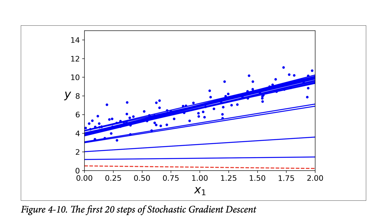
- Outer loop for
Important note on SGD (sidebar, page 126):
- Training instances must be independent and identically distributed (IID) for SGD to converge to global optimum on average.
- Shuffle instances during training (pick randomly, or shuffle set at start of each epoch). If data is sorted (e.g., by label), SGD will optimize for one label, then the next, and not find global minimum.
SGD with Scikit-Learn (
SGDRegressor, page 126):- Defaults to optimizing MSE.
sgd_reg = SGDRegressor(max_iter=1000, tol=1e-3, penalty=None, eta0=0.1)max_iter: max epochs.tol: stop if loss drops by less than this in one epoch.penalty=None: no regularization (more later).eta0: initial learning rate. Uses its own default learning schedule.
sgd_reg.fit(X, y.ravel())(.ravel()flattensyinto 1D array, often needed by Scikit-Learn).- Resulting intercept and coefficient are very close to Normal Equation’s.
Mini-batch Gradient Descent
A compromise between Batch GD and Stochastic GD.
- At each step, computes gradients on small random sets of instances called mini-batches.
- Main advantage over SGD: Performance boost from hardware optimization of matrix operations (especially on GPUs).
- Behavior (Figure 4-11, page 127):
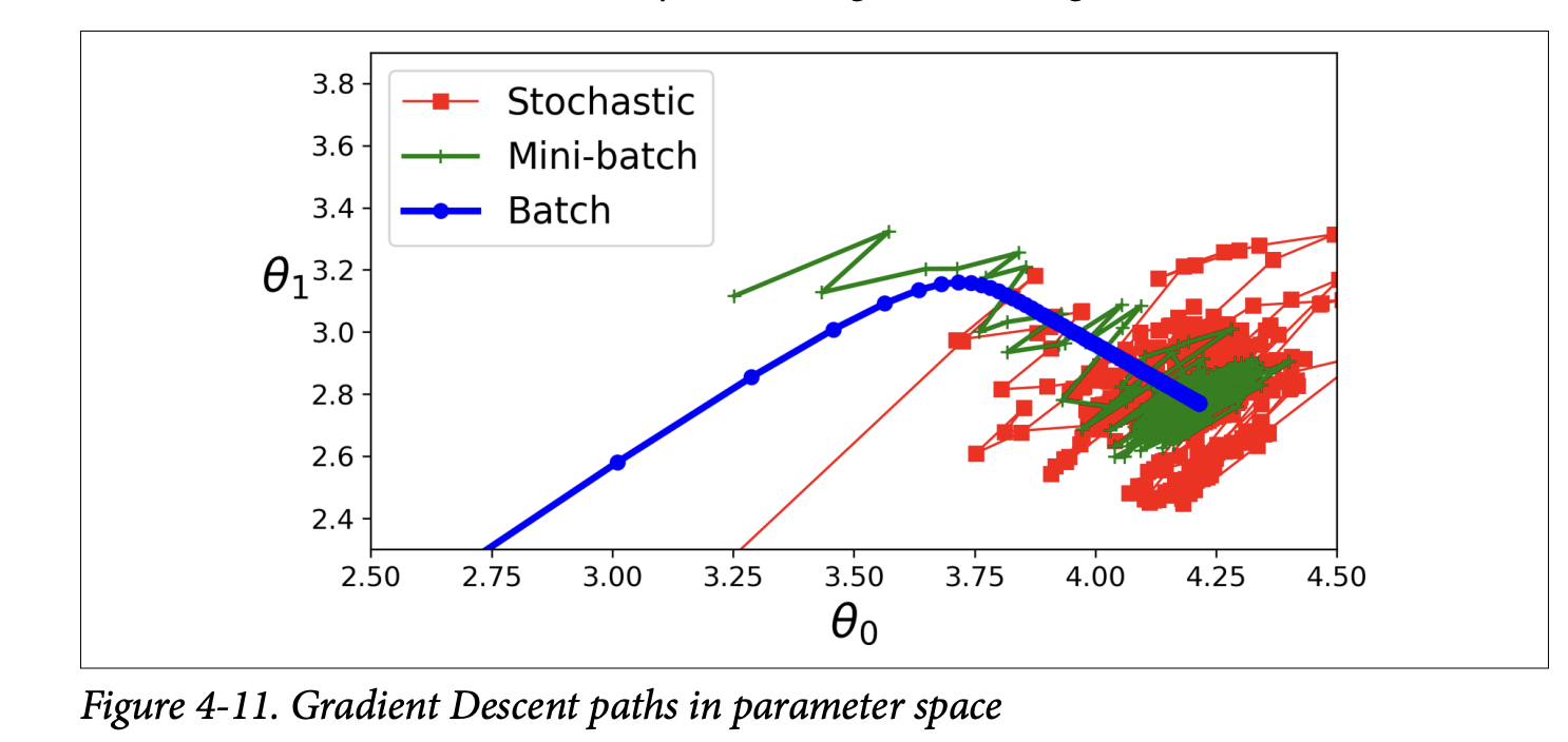
- Less erratic path than SGD.
- Ends up closer to the minimum than SGD (with fixed
η). - But may be harder to escape local minima (for non-convex problems) compared to SGD.
- All three (Batch, Stochastic, Mini-batch) end up near the minimum. Batch stops at the minimum. SGD and Mini-batch would also reach minimum with a good learning schedule.
- But Batch GD takes much longer per step.
Comparison Table 4-1
This table nicely summarizes Normal Equation, SVD, Batch GD, Stochastic GD, Mini-batch GD for Linear Regression based on:
Large m(instances): Normal Eq/SVD are fast if data fits memory. GD methods are also fast (SGD/Mini-batch can do out-of-core).Out-of-core support: Only SGD/Mini-batch.Large n(features): Normal Eq/SVD are slow. GD methods are fast.Hyperparameters: Normal Eq/SVD have 0. BGD has 2 (η, iterations). SGD/Mini-batch have >=2 (η, iterations, schedule params).Scaling required: No for Normal Eq/SVD. Yes for GD methods.Scikit-Learn class:LinearRegressionfor SVD.SGDRegressorfor GDs.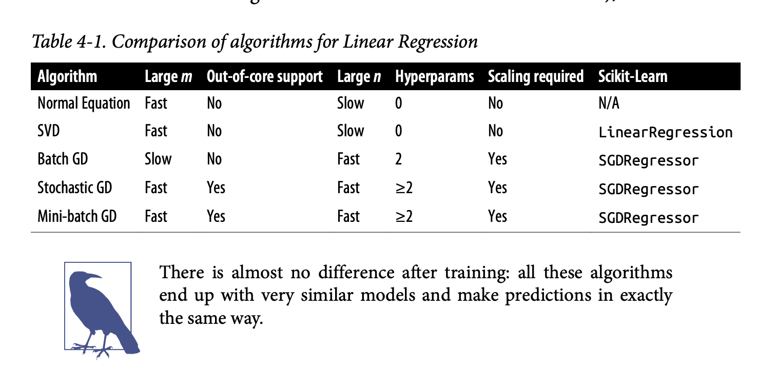
The key is that after training, all these methods (if converged) produce very similar models and make predictions in the same way. The difference is in how they get there (the training process).
Excellent! Glad you’re with me. Let’s push on to the next sections of Chapter 4. We’ve just laid the groundwork for how Linear Regression models are trained. Now, let’s see how we can adapt these ideas for more complex scenarios.
Polynomial Regression
So far, Linear Regression assumes a straight-line (or flat plane/hyperplane) relationship between features and the target. But what if your data is more complex, like the curved data in Figure 4-12 (page 129)?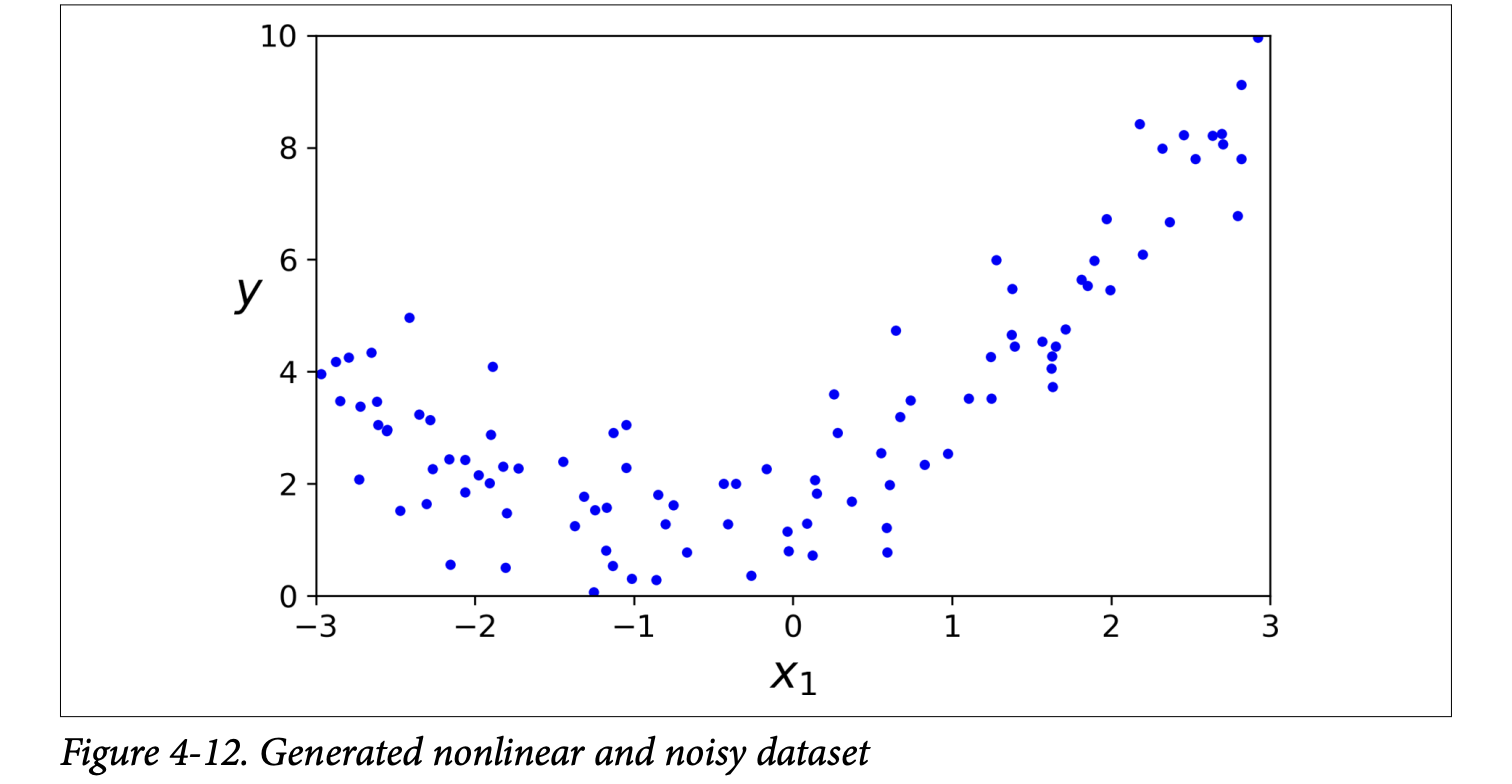
y = 0.5 * X2 + X + 2 + noise. Clearly, a straight line won’t fit this well.
This is where Polynomial Regression comes in.
The Core Idea: You can still use a linear model to fit nonlinear data!
How? By adding powers of each feature as new features, and then training a linear model on this extended set of features.
- For example, if you have one feature
X, you can create a new featureX². Then your linear model becomesŷ = θ₀ + θ₁X + θ₂X². Even though the equation is quadratic inX, it’s linear in terms of the parametersθ₀, θ₁, θ₂and the featuresXandX².
- For example, if you have one feature
Scikit-Learn’s
PolynomialFeatures(page 129): This class transforms your data.from sklearn.preprocessing import PolynomialFeaturespoly_features = PolynomialFeatures(degree=2, include_bias=False)degree=2: We want to add 2nd-degree polynomial features (i.e., squares).include_bias=False:PolynomialFeaturescan add a column of 1s (for the bias term), butLinearRegressionhandles that, so we set it toFalseto avoid redundancy.X_poly = poly_features.fit_transform(X)IfX[0]was[-0.75], thenX_poly[0]becomes[-0.75, 0.566](original X, and X²).
Train a Linear Model on Extended Data: Now, you just fit a standard
LinearRegressionmodel to thisX_poly:lin_reg = LinearRegression()lin_reg.fit(X_poly, y)The model predictions are shown in Figure 4-13 (page 130). It’s a nice curve that fits the data much better than a straight line! The estimated equation (e.g.,ŷ = 0.56x₁² + 0.93x₁ + 1.78) is close to the originaly = 0.5x₁² + 1.0x₁ + 2.0 + noise.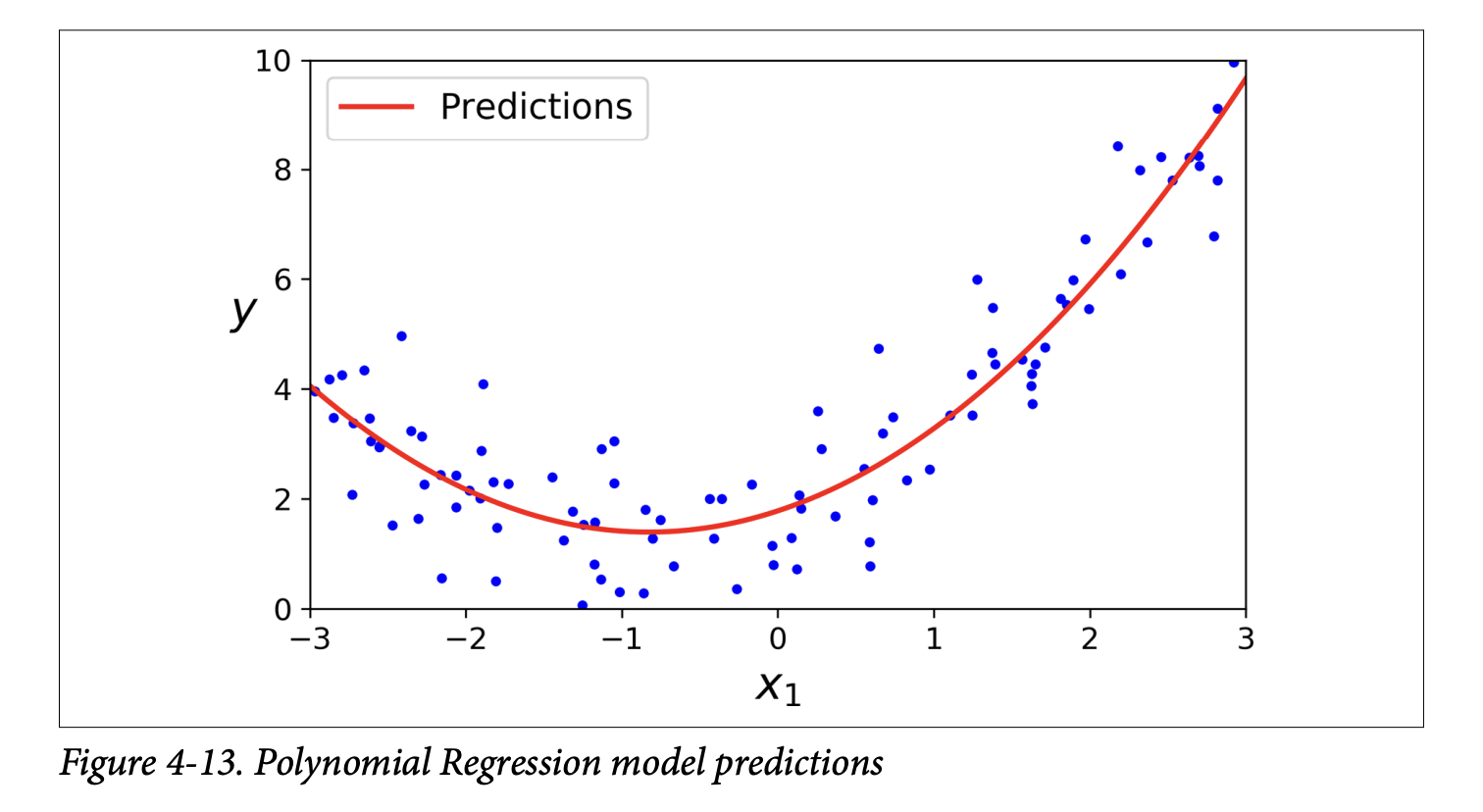
Multiple Features and Combinations (page 130): If you have multiple features (say,
aandb) and usePolynomialFeatures(degree=3), it will adda²,a³,b²,b³, AND also the combination terms likeab,a²b,ab². This allows the model to find relationships between features.Warning: Combinatorial Explosion! (Scorpion icon, page 130) The number of features can explode if you have many original features and use a high polynomial degree. The formula is
(n+d)! / (d!n!)wherenis original features,dis degree. Be careful! This can make the model very slow and prone to overfitting.
Learning Curves
With high-degree Polynomial Regression, you can fit the training data very well, maybe too well. Figure 4-14 (page 131) shows: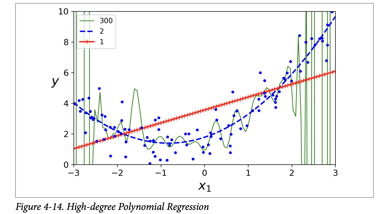
- A 300-degree polynomial model: Wiggles wildly to hit every training point. This is severe overfitting.
- A plain linear model: Misses the curve. This is underfitting.
- A quadratic model (2nd degree): Fits best, which makes sense as the data was generated quadratically.
But how do you know in general if your model is too complex (overfitting) or too simple (underfitting), especially if you don’t know the true underlying function?
Cross-Validation (from Chapter 2):
- If model performs well on training data but poorly on cross-validation, it’s overfitting.
- If it performs poorly on both, it’s underfitting.
Learning Curves (page 131):
What they are: Plots of the model’s performance (e.g., RMSE) on the training set and the validation set, as a function of the training set size (or training iteration).
How to generate them: Train the model multiple times on different-sized subsets of the training set.
The book provides a
plot_learning_curvesfunction (page 132).Learning Curves for an Underfitting Model (e.g., plain Linear Regression on the quadratic data - Figure 4-15, page 132):
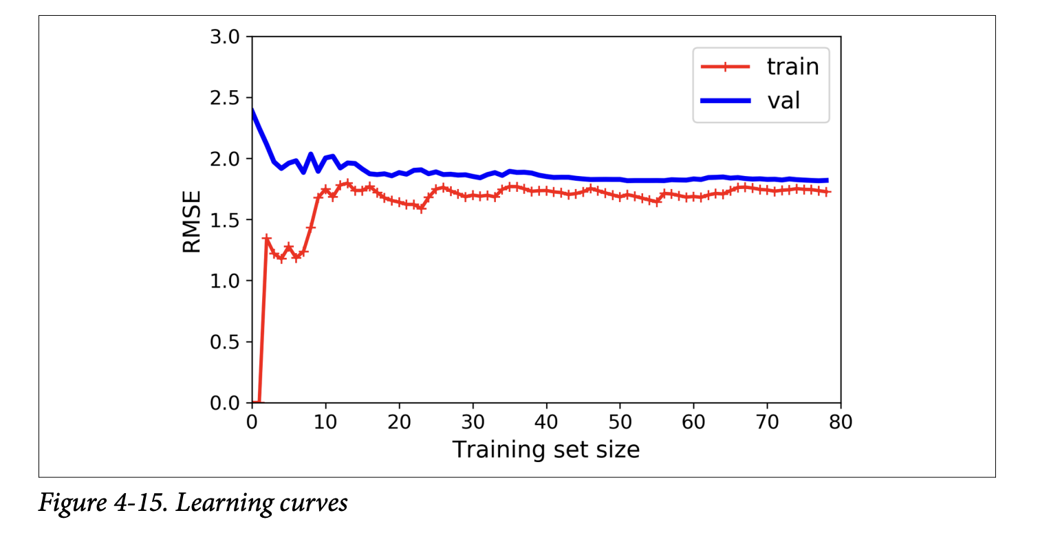
- Training error: Starts at 0 (perfect fit with 1-2 instances), then rises as more noisy/nonlinear data is added, eventually plateauing.
- Validation error: Starts very high (model trained on few instances generalizes poorly), then decreases as model learns from more examples, eventually plateauing close to the training error.
- Key characteristics of underfitting curves: Both curves plateau, they are close together, and the error is fairly high.
- What it’s ultimately trying to achieve: The plot tells you that the model is too simple. Adding more training examples will not help if the curves have plateaued (as the scorpion icon on page 133 says). You need a more complex model or better features.
Learning Curves for an Overfitting Model (e.g., 10th-degree polynomial on the quadratic data - Figure 4-16, page 133):
- Training error: Much lower than the Linear Regression model’s training error. It fits the training data well.
- Validation error: There’s a gap between the training error and the validation error. The model performs significantly better on the training data than on the validation data. This is the hallmark of overfitting.
- If you had a much larger training set, these two curves would eventually get closer.
- What it’s ultimately trying to achieve: The plot tells you the model is too complex for the current amount of data. One way to improve an overfitting model is to feed it more training data (as the scorpion icon on page 134 suggests), until the validation error meets the training error (or use regularization, which we’ll see next).
The Bias/Variance Trade-off (sidebar, page 134): This is a fundamental concept in statistics and ML. A model’s generalization error (how well it performs on unseen data) can be expressed as the sum of three components:
- Bias:
- Error due to wrong assumptions made by the model. E.g., assuming data is linear when it’s quadratic.
- A high-bias model is likely to underfit.
- What it’s ultimately trying to achieve (in a bad way): It has a strong preconceived notion of how the data should look, and it sticks to it even if the data says otherwise.
- Variance:
- Error due to the model’s excessive sensitivity to small variations in the training data. A model with many degrees of freedom (like a high-degree polynomial) can have high variance.
- A high-variance model is likely to overfit. It learns the noise in the training data, not just the signal.
- What it’s ultimately trying to achieve (in a bad way): It tries to fit every little nook and cranny of the training data, making it unstable and perform poorly on new, slightly different data.
- Irreducible Error:
- Error due to the inherent noisiness of the data itself.
- This part cannot be reduced by model changes; only by cleaning the data (e.g., fixing broken sensors, removing outliers).
The Trade-off:
- Increasing model complexity typically increases variance (more likely to overfit) and reduces bias (better fit to complex patterns).
- Decreasing model complexity typically increases bias (more likely to underfit) and reduces variance. The goal is to find a sweet spot, balancing bias and variance.
- Bias:
Regularized Linear Models
We saw that overfitting is a problem with complex models. Regularization is a way to reduce overfitting by constraining the model.
- What it’s ultimately trying to achieve: For linear models, this usually means constraining the model’s weights. The idea is to prevent the weights from becoming too large, which can happen when the model tries too hard to fit the noise in the training data. Smaller weights generally lead to simpler, smoother models that generalize better.
The book discusses three types of regularized linear models: Ridge, Lasso, and Elastic Net.
Ridge Regression (also Tikhonov regularization) (page 135):
- It adds a regularization term to the MSE cost function.
- Equation 4-8: Ridge Regression cost function
J(θ) = MSE(θ) + α * (1/2) * Σᵢ (θᵢ)²(sum from i=1 to n, so bias termθ₀is NOT regularized)- The regularization term is
α * (1/2) * Σᵢ (θᵢ)². This isα/2times the sum of the squares of the feature weights. This is related to the ℓ₂ norm of the weight vectorw = [θ₁, ..., θₙ], specifically(1/2) * ||w||₂². α(alpha) is a hyperparameter that controls how much you want to regularize.- If
α = 0, it’s just Linear Regression. - If
αis very large, all weightsθᵢ(for i>0) end up very close to zero, and the model becomes a flat line through the data’s mean.
- If
- What it’s ultimately trying to achieve: The learning algorithm is now forced to not only fit the data (minimize MSE) but also keep the model weights as small as possible.
- The regularization term is
- Important: Scale the data (e.g.,
StandardScaler) before performing Ridge Regression, as it’s sensitive to the scale of input features (scorpion icon, page 136). This is true for most regularized models. - Figure 4-17 (page 136) shows the effect of
α: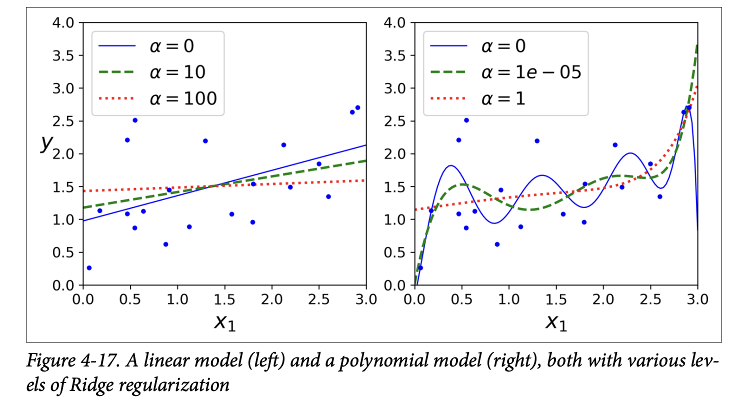
- Left: Plain Ridge Regression on linear data. Higher
αmakes predictions flatter. - Right: Polynomial features (degree=10) + scaling + Ridge. Increasing
αleads to flatter (less extreme, more reasonable) predictions, reducing variance but increasing bias.
- Left: Plain Ridge Regression on linear data. Higher
- Training Ridge Regression:
- Closed-form solution (Equation 4-9, page 137):
θ̂ = (XᵀX + αA)⁻¹ Xᵀy(whereAis an identity matrix with a 0 at the top-left for the bias term). Scikit-Learn’sRidge(alpha=..., solver="cholesky")uses this. - Gradient Descent (page 137):
Add
αwto the MSE gradient vector (wherewis the vector of weights, excluding bias). Scikit-Learn’sSGDRegressor(penalty="l2")does this. The"l2"means add a regularization term equal to half the square of the ℓ₂ norm of the weights.
- Closed-form solution (Equation 4-9, page 137):
Lasso Regression (Least Absolute Shrinkage and Selection Operator) (page 137):
- Also adds a regularization term to the MSE cost function, but uses the ℓ₁ norm of the weight vector.
- Equation 4-10: Lasso Regression cost function
J(θ) = MSE(θ) + α * Σᵢ |θᵢ|(sum from i=1 to n)- The regularization term is
αtimes the sum of the absolute values of the weights.
- The regularization term is
- Figure 4-18 (page 138) shows Lasso models, similar to Figure 4-17 for Ridge, but with smaller
αvalues.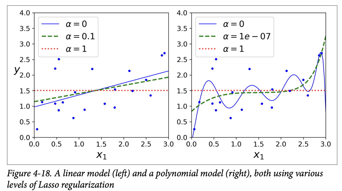
- Key characteristic of Lasso: It tends to completely eliminate the weights of the least important features (i.e., set them to zero). It automatically performs feature selection and outputs a sparse model (a model with few non-zero feature weights).
- Why does Lasso do this? (Figure 4-19, page 139):
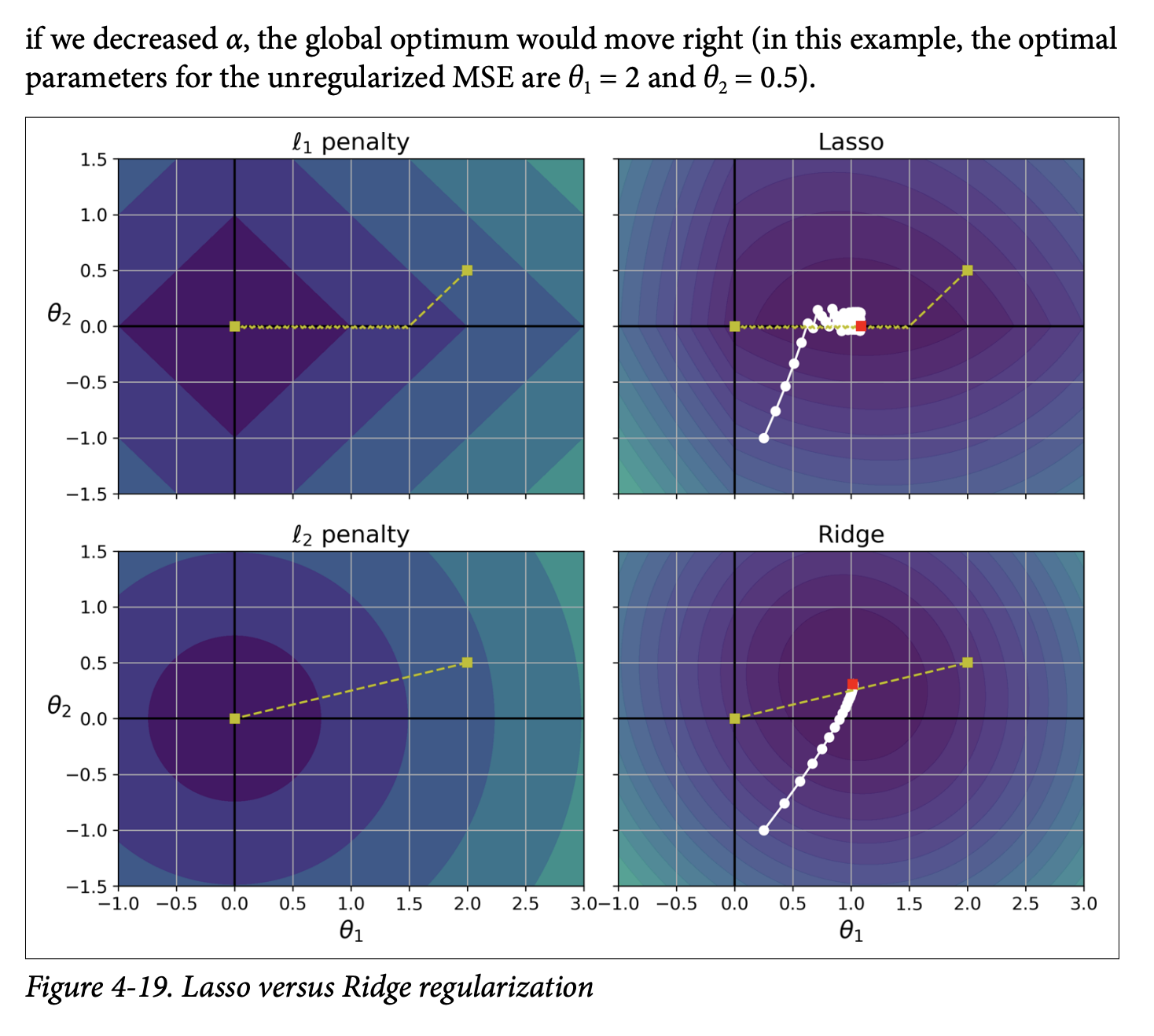
- This is a bit more advanced, but the intuition comes from looking at the “shape” of the ℓ₁ penalty vs. the ℓ₂ penalty.
- The ℓ₁ penalty
|θ₁| + |θ₂|has “corners” along the axes in the parameter space. When minimizing the combined MSE + ℓ₁ penalty, the optimization path often hits these corners, forcing one of the parameters to zero. - The ℓ₂ penalty
θ₁² + θ₂²is circular. The optimization path approaches the origin smoothly, shrinking weights but not usually making them exactly zero. - What it’s ultimately trying to achieve: The ℓ₁ penalty encourages sparsity by pushing less important feature weights all the way to zero.
- Training Lasso Regression:
- The Lasso cost function is not differentiable at
θᵢ = 0. However, Gradient Descent can still work if you use a subgradient vector (Equation 4-11, page 140). This is a technical detail; the main idea is that an iterative approach can still find the minimum. - Scikit-Learn:
Lasso(alpha=...)orSGDRegressor(penalty="l1"). - When using Lasso with GD, you often need to gradually reduce the learning rate to help it converge without bouncing around the optimum (due to the “sharp corners” of the ℓ₁ penalty).
- The Lasso cost function is not differentiable at
Elastic Net (page 140):
- A middle ground between Ridge and Lasso. Its regularization term is a simple mix of both Ridge (ℓ₂) and Lasso (ℓ₁) terms.
- Equation 4-12: Elastic Net cost function
J(θ) = MSE(θ) + rα Σᵢ|θᵢ| + ((1-r)/2)α Σᵢθᵢ²ris the mix ratio.- If
r = 0, Elastic Net is equivalent to Ridge. - If
r = 1, Elastic Net is equivalent to Lasso.
- If
- Scikit-Learn:
ElasticNet(alpha=..., l1_ratio=...)(wherel1_ratioisr).
When to use which? (page 140):
- Plain Linear Regression (no regularization) should generally be avoided. Some regularization is almost always better.
- Ridge is a good default.
- If you suspect only a few features are useful, prefer Lasso or Elastic Net because they perform feature selection by shrinking useless feature weights to zero.
- Elastic Net is generally preferred over Lasso because Lasso can behave erratically when the number of features is greater than the number of training instances, or when several features are strongly correlated. Elastic Net is more stable in these cases.
Early Stopping (page 141):
- A very different way to regularize iterative learning algorithms like Gradient Descent.
- The Idea: Stop training as soon as the validation error reaches a minimum.
- Figure 4-20 (page 141) shows a complex model (high-degree polynomial) being trained with Batch GD:
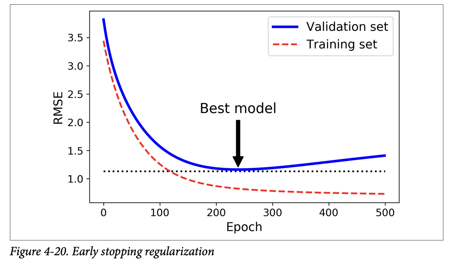
- As epochs go by, training error (RMSE) goes down.
- Validation error also goes down initially, but then starts to go back up. This indicates the model has started to overfit.
- With early stopping, you just stop training when the validation error is at its minimum.
- It’s a simple and efficient regularization technique. Geoffrey Hinton called it a “beautiful free lunch.”
- Implementation (page 142):
- Loop for epochs.
- In each epoch, train the model (e.g.,
SGDRegressorwithwarm_start=Trueso it continues training,max_iter=1so it does one epoch). - Evaluate on validation set.
- If validation error is less than current
minimum_val_error, save the model (clone it) and updateminimum_val_errorandbest_epoch. - After the loop, the
best_modelis your regularized model.
- With SGD/Mini-batch GD, validation curves are noisy. You might stop only after validation error has been above minimum for a while, then roll back to the best model.
Fantastic! It’s great that the intuition behind L1 and L2 regularization clicked. Let’s continue our journey through Chapter 4, moving on to models designed for classification.
Logistic Regression
We’ve seen Linear Regression for predicting continuous values. Now, what if we want to predict a class? For example, is an email spam or not spam? This is a binary classification problem.
The book points out (as we saw in Chapter 1) that some regression algorithms can be adapted for classification. Logistic Regression (also called Logit Regression) is a prime example.
What it’s ultimately trying to achieve: Logistic Regression estimates the probability that an instance belongs to a particular class (typically the “positive” class, labeled ‘1’). If this probability is greater than a certain threshold (usually 50%), the model predicts ‘1’; otherwise, it predicts ‘0’.
Estimating Probabilities (Page 143):
- Linear Combination: Just like Linear Regression, it first computes a weighted sum of the input features plus a bias term:
t = xᵀθ. (Thistis often called the logit). - Logistic Function (Sigmoid): Instead of outputting
tdirectly, it passestthrough the logistic function (also called the sigmoid function), denoted asσ(t).- Equation 4-13: Logistic Regression model estimated probability (vectorized form)
p̂ = h_θ(x) = σ(xᵀθ)wherep̂(p-hat) is the estimated probability that the instancexbelongs to the positive class. - Equation 4-14: Logistic function
σ(t) = 1 / (1 + exp(-t)) - Figure 4-21 (page 143) shows the characteristic S-shape of the sigmoid function.
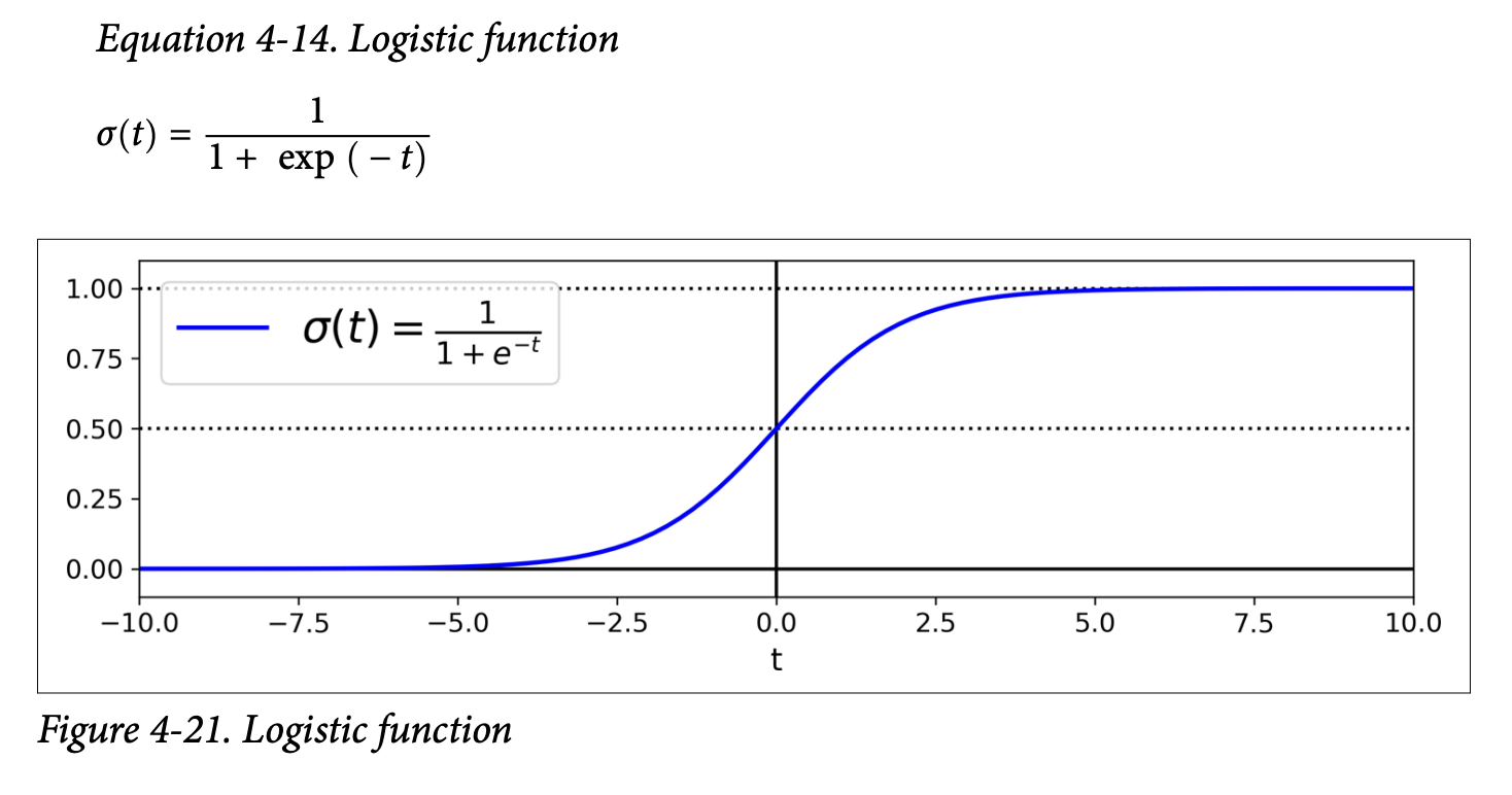
- What the sigmoid is ultimately trying to achieve: It squashes any input value
t(which can range from -∞ to +∞) into an output value between 0 and 1. This output can then be interpreted as a probability.- If
tis large and positive,exp(-t)is close to 0, soσ(t)is close to 1. - If
tis large and negative,exp(-t)is very large, soσ(t)is close to 0. - If
t = 0,exp(-t) = 1, soσ(t) = 1/2 = 0.5.
- If
- What the sigmoid is ultimately trying to achieve: It squashes any input value
- Equation 4-13: Logistic Regression model estimated probability (vectorized form)
- Linear Combination: Just like Linear Regression, it first computes a weighted sum of the input features plus a bias term:
Making Predictions (Page 143):
- Equation 4-15: Logistic Regression model prediction
ŷ = 0 if p̂ < 0.5ŷ = 1 if p̂ ≥ 0.5 - Since
σ(t) ≥ 0.5whent ≥ 0, the model predicts 1 ifxᵀθ(the logit) is positive, and 0 if it’s negative.
- Equation 4-15: Logistic Regression model prediction
Training and Cost Function (Page 144):
- Objective: We want to set the parameter vector
θso that the model estimates a high probability for positive instances (actual y=1) and a low probability for negative instances (actual y=0). - Cost Function for a Single Instance (Equation 4-16):
c(θ) = -log(p̂) if y = 1c(θ) = -log(1 - p̂) if y = 0- What this cost function is ultimately trying to achieve:
- If
y=1(actual is positive):- If model predicts
p̂close to 1 (correct),-log(p̂)is close to 0 (low cost). - If model predicts
p̂close to 0 (incorrect),-log(p̂)is very large (high cost).
- If model predicts
- If
y=0(actual is negative):- If model predicts
p̂close to 0 (so1-p̂is close to 1, correct),-log(1-p̂)is close to 0 (low cost). - If model predicts
p̂close to 1 (so1-p̂is close to 0, incorrect),-log(1-p̂)is very large (high cost). This cost function penalizes the model heavily when it’s confident and wrong.
- If model predicts
- If
- What this cost function is ultimately trying to achieve:
- Cost Function for the Whole Training Set (Log Loss - Equation 4-17):
J(θ) = - (1/m) * Σᵢ [ y⁽ⁱ⁾log(p̂⁽ⁱ⁾) + (1 - y⁽ⁱ⁾)log(1 - p̂⁽ⁱ⁾) ]This is just the average cost over all training instances. It’s a single, clever expression that combines the two cases from Equation 4-16. - Good news: This log loss cost function is convex. So, Gradient Descent (or other optimization algorithms) can find the global minimum.
- Bad news: There’s no closed-form solution (like the Normal Equation for Linear Regression) to find the
θthat minimizes this cost function. We must use an iterative optimization algorithm like Gradient Descent. - Partial Derivatives (Equation 4-18, page 145):
∂J(θ)/∂θⱼ = (1/m) * Σᵢ (σ(θᵀx⁽ⁱ⁾) - y⁽ⁱ⁾) * xⱼ⁽ⁱ⁾- This looks very similar to the partial derivative for Linear Regression’s MSE (Equation 4-5)!
σ(θᵀx⁽ⁱ⁾)is the predicted probabilityp̂⁽ⁱ⁾.(p̂⁽ⁱ⁾ - y⁽ⁱ⁾)is the prediction error.- This error is multiplied by the feature value
xⱼ⁽ⁱ⁾and averaged. Once you have these gradients, you can use Batch GD, Stochastic GD, or Mini-batch GD to find the optimalθ.
- Objective: We want to set the parameter vector
Decision Boundaries (Page 145-147): Let’s use the Iris dataset to illustrate. We’ll try to classify Iris virginica based only on petal width.
- Load data:
X = iris["data"][:, 3:](petal width),y = (iris["target"] == 2).astype(int)(1 if virginica, else 0). - Train
LogisticRegression():log_reg = LogisticRegression()log_reg.fit(X, y) - Figure 4-23 (page 146): Shows estimated probabilities vs. petal width.
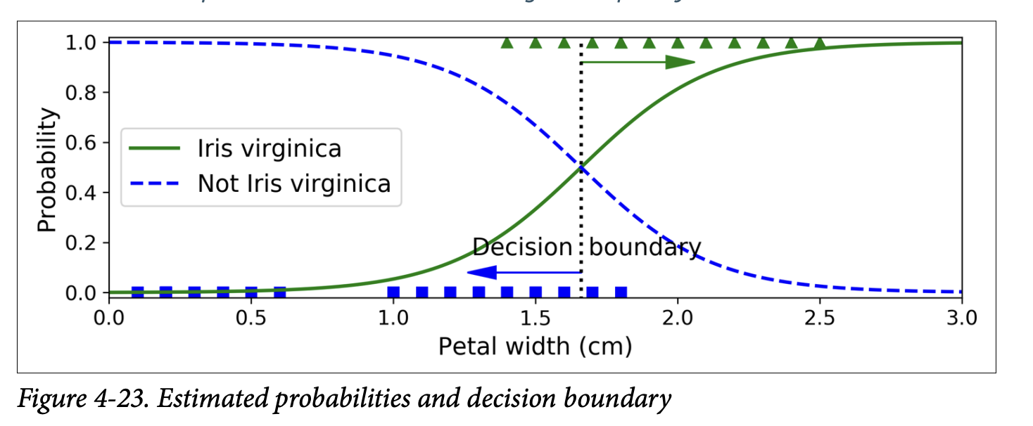
- The S-shape is clear.
- For petal widths > ~2cm, probability of being Iris virginica is high.
- For petal widths < ~1cm, probability is low.
- The decision boundary (where
p̂ = 0.5) is around 1.6 cm. If petal width > 1.6cm, it predicts virginica; otherwise, not virginica.
- Figure 4-24 (page 147): Shows decision boundary using two features (petal width and petal length).
- The dashed line is where the model estimates 50% probability – this is the linear decision boundary.
- Other parallel lines show other probability contours (e.g., 15%, 90%).
- Regularization: Logistic Regression models in Scikit-Learn use ℓ₂ regularization by default. The hyperparameter is
C(inverse ofα): higherCmeans less regularization.
- Load data:
Softmax Regression
Logistic Regression is for binary classification. What if we have more than two classes, and we want a model that handles them directly (not with OvR/OvO strategies)? Enter Softmax Regression (or Multinomial Logistic Regression).
The Idea:
- For a given instance
x, compute a scoresₖ(x)for each classk. This is done just like Linear Regression:sₖ(x) = xᵀθ⁽ᵏ⁾(Equation 4-19). Each classkhas its own dedicated parameter vectorθ⁽ᵏ⁾. These are often stored as rows in a parameter matrixΘ. - Estimate the probability
p̂ₖthat the instance belongs to classkby applying the softmax function (also called normalized exponential) to the scores.- Equation 4-20: Softmax function
p̂ₖ = σ(s(x))ₖ = exp(sₖ(x)) / Σⱼ exp(sⱼ(x))(sum over all classesj=1toK)- What it’s ultimately trying to achieve: It takes a vector of arbitrary scores
s(x)for all classes, computes the exponential of each score (making them all positive), and then normalizes them by dividing by their sum. The result is a set of probabilities (p̂ₖ) that are all between 0 and 1 and sum up to 1 across all classes. The class with the highest initial scoresₖ(x)will get the highest probabilityp̂ₖ.
- What it’s ultimately trying to achieve: It takes a vector of arbitrary scores
- Equation 4-20: Softmax function
- For a given instance
Prediction (Equation 4-21, page 149): The classifier predicts the class
kthat has the highest estimated probabilityp̂ₖ(which is simply the class with the highest scoresₖ(x)).ŷ = argmaxₖ p̂ₖ- Softmax Regression predicts only one class at a time (mutually exclusive classes). It’s multiclass, not multioutput.
Training and Cost Function (Cross Entropy - page 149):
- Objective: Estimate a high probability for the target class and low probabilities for other classes.
- Cost Function (Cross Entropy - Equation 4-22):
J(Θ) = - (1/m) * Σᵢ Σₖ yₖ⁽ⁱ⁾ log(p̂ₖ⁽ⁱ⁾)yₖ⁽ⁱ⁾is the target probability that instanceibelongs to classk(usually 1 if it’s the target class, 0 otherwise).p̂ₖ⁽ⁱ⁾is the model’s estimated probability that instanceibelongs to classk.- What it’s ultimately trying to achieve: This cost function penalizes the model when it estimates a low probability for the actual target class. It’s a common measure for how well a set of estimated class probabilities matches the target classes.
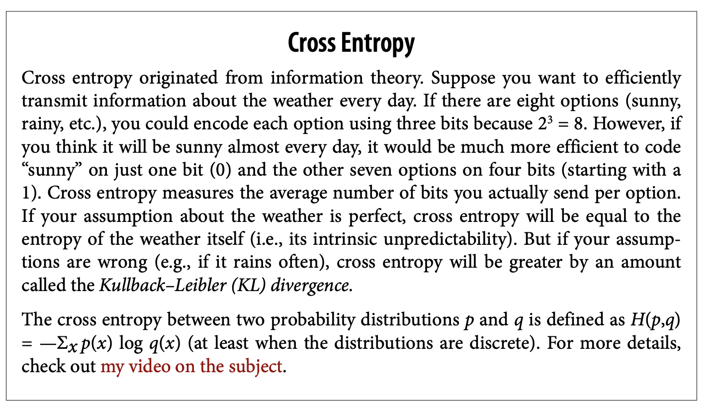
- The sidebar on “Cross Entropy” (page 150) gives some information theory background – it measures the average number of bits needed to encode events based on your probability estimates vs. the true probabilities. Lower is better.
- When there are only two classes (K=2), this cross-entropy cost function is equivalent to the log loss for Logistic Regression.
- Gradient Vector (Equation 4-23, page 150):
∇_θ⁽ᵏ⁾ J(Θ) = (1/m) * Σᵢ (p̂ₖ⁽ⁱ⁾ - yₖ⁽ⁱ⁾) * x⁽ⁱ⁾This gives the gradient for the parameter vectorθ⁽ᵏ⁾of a specific classk. Again, very similar form to previous gradient equations! You compute this for every class, then use an optimization algorithm (like GD) to find the parameter matrixΘthat minimizes the cost.
Using Softmax Regression in Scikit-Learn (page 150):
LogisticRegressioncan perform Softmax Regression by setting:multi_class="multinomial"solver="lbfgs"(or another solver that supports multinomial, like “sag” or “newton-cg”)- It also applies ℓ₂ regularization by default (controlled by
C).
- Example: Classify Iris flowers into all 3 classes using petal length and width.
X = iris["data"][:, (2, 3)]y = iris["target"]softmax_reg = LogisticRegression(multi_class="multinomial", solver="lbfgs", C=10)softmax_reg.fit(X, y) - To predict:
softmax_reg.predict([[5, 2]])might givearray([2])(Iris virginica). - To get probabilities:
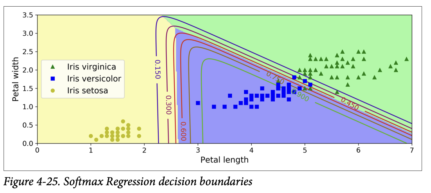
softmax_reg.predict_proba([[5, 2]])might give[[6.3e-07, 0.057, 0.942]], meaning 94.2% prob for class 2 (virginica), 5.8% for class 1 (versicolor), and near 0% for class 0 (setosa). - Figure 4-25 (page 151) shows the decision boundaries. They are linear between any two classes.
And that brings us to the end of the core content of Chapter 4! We’ve gone from simple Linear Regression to Polynomial Regression, learned about diagnosing model fit with learning curves, seen how to regularize models to prevent overfitting (Ridge, Lasso, Elastic Net, Early Stopping), and finally explored Logistic and Softmax Regression for classification tasks.
The recurring theme for training, especially for models without closed-form solutions, is defining a cost function that captures how “bad” our model is, and then using an iterative algorithm like Gradient Descent to find the model parameters that minimize this cost. The specific form of the cost function and how predictions are made change from model to model, but the underlying optimization principle is often very similar.
This chapter is dense, but the concepts are absolutely key for understanding how models actually learn. How are you feeling about Logistic and Softmax Regression? Any particular part of “what they are trying to achieve” that needs more light?
Glossary
Difference between L1 (Lasso) and L2 (Ridge) regularization! Let’s break down that intuition about the “shapes” and “corners.”
Imagine we have a model with just two weights, θ₁ and θ₂. We want to find the values of θ₁ and θ₂ that minimize our main cost function (let’s say MSE), subject to some penalty on the size of these weights.
Visualizing the Penalties (Loss Functions for Weights)
Think of the penalty term as defining a “budget” or a “constraint region” for our weights. The optimization process is trying to find the best MSE it can, while staying within or close to this budget defined by the penalty.
L₂ Penalty (Ridge):
θ₁² + θ₂² ≤ C- The equation
θ₁² + θ₂² = constantdescribes a circle (or a sphere/hypersphere in higher dimensions) centered at the origin (θ₁=0, θ₂=0). - So, the L2 penalty encourages the weights
(θ₁, θ₂)to stay within a circular region around the origin. - Shape: Smooth and round. No sharp corners.
- Imagine the contours of this penalty function: they are concentric circles.
- The equation
L₁ Penalty (Lasso):
|θ₁| + |θ₂| ≤ C- The equation
|θ₁| + |θ₂| = constantdescribes a diamond (or a rotated square in 2D, and a similar shape with “pointy” corners on the axes in higher dimensions). - So, the L1 penalty encourages the weights
(θ₁, θ₂)to stay within a diamond-shaped region around the origin. - Shape: Has sharp corners that lie on the axes. For our 2D example, the corners are at points like (C, 0), (-C, 0), (0, C), and (0, -C).
- Imagine the contours of this penalty function: they are concentric diamonds.
- The equation
Visualizing the Optimization Process (Figure 4-19)
Now, let’s consider the main cost function, the MSE. The contours of the MSE (if we ignore the penalty for a moment) are typically elliptical. The center of these ellipses is the point where MSE is minimized without any regularization – let’s call this the “unconstrained optimum.”
The regularization process is trying to find a point that: a. Is on the lowest possible MSE contour (meaning good fit to the data). b. Satisfies the “budget” imposed by the L1 or L2 penalty (meaning weights are small).
This can be visualized as finding the point where an MSE ellipse first “touches” the boundary of the penalty region (the circle for L2, the diamond for L1).
With L₂ Penalty (Ridge - bottom-right plot in Figure 4-19):
- Imagine an expanding MSE ellipse (as we try to get lower MSE) until it just kisses the circular L2 penalty region.
- Because the circle is smooth and round, the point where the ellipse touches it can be anywhere on the circle’s boundary.
- It’s very unlikely that this touch point will be exactly on an axis (e.g., where
θ₁ = 0orθ₂ = 0). - Result: The L2 penalty shrinks both
θ₁andθ₂towards zero, but it’s rare for either of them to become exactly zero. The optimization path (white dots) goes smoothly towards a point where both weights are small but likely non-zero.
With L₁ Penalty (Lasso - top-right plot in Figure 4-19):
- Imagine an expanding MSE ellipse until it just kisses the diamond-shaped L1 penalty region.
- Because the diamond has sharp corners on the axes, it’s much more likely that the ellipse will first touch the diamond at one of these corners.
- If it touches at a corner on, say, the
θ₁-axis, then at that point,θ₂will be exactly zero. - Result: The L1 penalty also shrinks weights towards zero, but because of its shape, it often forces some weights to become exactly zero. This is the “feature selection” property. The optimization path (white dots) is shown hitting the
θ₂=0axis and then “rolling down the gutter” along that axis.
Why the “Corners” Matter for Hitting Zero:
Think about the gradient (the direction of steepest descent) of the penalty term itself:
- L₂ Penalty: The gradient of
θ₁² + θ₂²always points directly towards the origin. It smoothly pulls all weights smaller. - L₁ Penalty: The gradient of
|θ₁| + |θ₂|is a bit trickier.- If
θ₁ > 0, the derivative w.r.t.θ₁is 1. - If
θ₁ < 0, the derivative w.r.t.θ₁is -1. - If
θ₁ = 0, it’s undefined (this is the “corner”). This means the L1 penalty applies a constant “force” (either +1 or -1) pulling a weight towards zero, regardless of how small the weight already is (as long as it’s not zero). Once a weight hits zero, this “force” can effectively keep it there if the pull from the MSE term isn’t strong enough to move it away. In contrast, for L2, the “force”2θ₁pullingθ₁towards zero gets weaker asθ₁gets smaller. So, it might get very close to zero but not quite hit it unless the MSE term also strongly favors zero.
- If
Intuitive Summary:
- L₂ (Ridge) is like saying: “Try to make your weights small, and distribute the ‘smallness’ somewhat evenly. Keep them inside this round ball.” It pulls weights towards zero but doesn’t aggressively zero them out.
- L₁ (Lasso) is like saying: “Try to make your weights small, and if possible, make some of them exactly zero. Keep them inside this pointy diamond. It’s okay to focus your ‘budget’ on just a few important weights and eliminate the others.”
The “corners” of the L1 penalty region are key because they represent solutions where one or more weights are exactly zero. The optimization process, in trying to balance minimizing MSE with staying within the L1 budget, often finds its optimal solution precisely at one of these corners.
Does that help clarify why the shape of the penalty (round vs. pointy with corners on axes) leads to these different behaviors in terms of zeroing out weights?
Okay, absolutely! Let’s revisit Softmax Regression (pages 148-150) and really focus on what it’s ultimately trying to achieve, especially in contrast to just using multiple binary Logistic Regressions.
You’re spot on: Logistic Regression is great for “is it A or not A?” (binary). But what if you have “is it A, B, C, or D?” (multiclass).
The Problem with Just Using Multiple Binary Classifiers (OvR/OvO):
We saw in Chapter 3 that you can use binary classifiers for multiclass problems:
One-vs-Rest (OvR): Train a separate binary Logistic Regression for each class.
- Classifier 1: “Is it class A (vs. B, C, D)?”
- Classifier 2: “Is it class B (vs. A, C, D)?”
- …and so on.
- To make a prediction, you run your input through all these binary classifiers and pick the class whose classifier gives the highest “confidence” score (or probability, if the binary classifier outputs that).
One-vs-One (OvO): Train a binary classifier for every pair of classes (A vs B, A vs C, A vs D, B vs C, etc.). Pick the class that wins the most “duels.”
Limitations/Quirks of OvR/OvO for Probabilities:
While these strategies work for getting a class label, there’s a slight awkwardness if you want well-calibrated probabilities for each class that naturally sum to 1.
- With OvR, each binary Logistic Regression outputs a probability for its class versus all others. For example,
P(A | not A). These probabilities from different classifiers aren’t inherently guaranteed to sum to 1 when you look across all classes for a single instance. You might getP(A)=0.7,P(B)=0.4,P(C)=0.1. These don’t sum to 1, and it’s not immediately clear how to turn them into a proper probability distribution over A, B, and C. You usually just pick the class with the highest score.
Softmax Regression: The “Direct” Multiclass Probabilistic Approach
Softmax Regression is designed from the ground up to handle multiple classes directly and produce a consistent set of probabilities that sum to 1 across all classes.
Here’s the core idea and “what it’s trying to achieve”:
Goal: For any given input instance (e.g., an image of a digit), we want to output a probability for each possible class (e.g., P(digit is 0), P(digit is 1), …, P(digit is 9)). Critically, these probabilities should all add up to 100%.
Step 1: Calculate a “Score” for Each Class (Equation 4-19)
- Just like Linear Regression or Logistic Regression, for each class
k, Softmax Regression calculates a linear score:sₖ(x) = xᵀθ⁽ᵏ⁾ xis the input feature vector.θ⁽ᵏ⁾(theta-k) is a separate vector of weights specifically for classk. So, if you have 10 classes (digits 0-9), you will have 10 differentθvectors.- What these scores
sₖ(x)are ultimately trying to achieve: They are like raw “evidence” or “suitability scores” for each class, given the inputx. A higher scoresₖ(x)suggests that classkis a more likely candidate for this input. These scores can be any real number (positive, negative, large, small).
- Just like Linear Regression or Logistic Regression, for each class
Step 2: Convert Scores into Probabilities (The Softmax Function - Equation 4-20)
- The raw scores
sₖ(x)are not probabilities yet (they don’t sum to 1, and they can be negative). We need a way to transform them into a valid probability distribution. This is where the softmax function (also called “normalized exponential”) comes in. - For each class
k, the probabilityp̂ₖis calculated as:p̂ₖ = exp(sₖ(x)) / Σⱼ exp(sⱼ(x))(where the sum in the denominator is over all possible classesj) - What the softmax function is ultimately trying to achieve:
exp(sₖ(x))(Exponential): First, it takes the exponential of each score. This has two effects:- It makes all scores positive (since
eto any power is positive). - It tends to exaggerate differences: if score A is slightly higher than score B,
exp(A)will be significantly higher thanexp(B). The “softmax” is “soft” in that it doesn’t just pick the max score and give it 100% probability, but it does give more weight to higher scores.
- It makes all scores positive (since
Σⱼ exp(sⱼ(x))(Sum of Exponentials): It then sums up these positive, exponentiated scores for all classes. This sum acts as a normalization constant.- Division: Dividing each
exp(sₖ(x))by this total sum ensures two things:- Each
p̂ₖwill be between 0 and 1. - All the
p̂ₖvalues will sum up to 1. So, we get a proper probability distribution across all classes. The class that had the highest initial scoresₖ(x)will end up with the largest probabilityp̂ₖ.
- Each
- The raw scores
Analogy for Softmax:
Imagine you have several candidates for a job (the classes).
- You give each candidate a raw “suitability score” (the
sₖ(x)). Some might be high, some low, some even negative if they seem really unsuitable. - To decide how to allocate a “probability of being hired” that sums to 100% across all candidates:
- You first want to ensure everyone’s considered “positively” and amplify the scores of strong candidates: you “exponentiate” their scores. A candidate with a score of 3 becomes
e³ ≈ 20, while a candidate with a score of 1 becomese¹ ≈ 2.7. The difference is magnified. - Then, you add up all these amplified, positive scores to get a “total pool of amplified suitability.”
- Finally, each candidate’s share of this total pool becomes their probability of being hired.
- You first want to ensure everyone’s considered “positively” and amplify the scores of strong candidates: you “exponentiate” their scores. A candidate with a score of 3 becomes
Why is this better than just running multiple OvR Logistic Regressions for probabilities?
- Direct Probabilistic Interpretation: Softmax directly outputs a set of probabilities that are inherently linked and sum to 1. It’s designed for this purpose. With OvR Logistic Regression, you’d have to do some extra (potentially ad-hoc) normalization step if you wanted the “probabilities” from different binary classifiers to sum to 1 for a given instance.
- Shared Information During Training (via the cost function): When Softmax Regression is trained (using the cross-entropy cost function, which we’ll get to), the updates to the weights
θ⁽ᵏ⁾for one class are influenced by the scores and target probabilities of all other classes because of that denominator in the softmax function. This allows the model to learn the relationships and distinctions between all classes simultaneously in a more coupled way. With independent OvR classifiers, each classifier only learns to distinguish its class from “everything else” without explicitly considering the fine-grained distinctions between those “everything else” classes.
Making a Prediction and Training:
- Prediction (Equation 4-21): Once you have the probabilities
p̂ₖfor all classes, you simply predict the classkthat has the highest probability. This is equivalent to picking the class with the highest initial scoresₖ(x). - Training (Cross-Entropy Cost Function - Equation 4-22):
- The goal is to find the parameter matrix
Θ(which contains all theθ⁽ᵏ⁾vectors) such that for a given training instance, the predicted probabilityp̂ₖis high for the correct classkand low for all other classes. - The cross-entropy cost function is used for this.
J(Θ) = - (1/m) * Σᵢ Σₖ yₖ⁽ⁱ⁾ log(p̂ₖ⁽ⁱ⁾)yₖ⁽ⁱ⁾is 1 if classkis the true class for instancei, and 0 otherwise.- What it’s ultimately trying to achieve: It heavily penalizes the model if
log(p̂ₖ⁽ⁱ⁾)is a large negative number for the true classk(which happens ifp̂ₖ⁽ⁱ⁾is close to 0 for the true class). It wants to maximize the log-probability of the correct class.
- This cost function is convex, so Gradient Descent can find the optimal
Θ. The gradients (Equation 4-23) are computed, andΘis updated iteratively.
- The goal is to find the parameter matrix
In essence, Softmax Regression is a generalization of Logistic Regression to handle multiple classes by:
- Calculating a linear score for each class.
- Using the softmax function to convert these scores into a proper probability distribution over all classes.
- Being trained with a cost function (cross-entropy) that encourages high probabilities for correct classes.
It provides a more principled and direct way to get multiclass probabilities compared to trying to combine multiple independent binary logistic regressions.
Focus on the Cross-Entropy cost function
Let’s break it down slowly, focusing on what it’s ultimately trying to achieve.
Recall the equation:
J(Θ) = - (1/m) * Σᵢ Σₖ yₖ⁽ⁱ⁾ log(p̂ₖ⁽ⁱ⁾)
Where:
J(Θ): The total cost for our model parametersΘ. We want to minimize this.m: The number of training instances.(1/m)means we’re averaging the cost over all instances.Σᵢ: Sum over all training instancesi(from 1 tom).Σₖ: Sum over all possible classesk(from 1 toK).yₖ⁽ⁱ⁾: This is the true target probability that instanceibelongs to classk.- For most classification problems (like digit recognition), this is a “one-hot encoded” value. If instance
iis truly a ‘digit 3’, then:y₃⁽ⁱ⁾ = 1(the probability of being class ‘3’ is 100%)y₀⁽ⁱ⁾ = 0,y₁⁽ⁱ⁾ = 0,y₂⁽ⁱ⁾ = 0,y₄⁽ⁱ⁾ = 0, …,y₉⁽ⁱ⁾ = 0(the probability of being any other class is 0%).
- For most classification problems (like digit recognition), this is a “one-hot encoded” value. If instance
p̂ₖ⁽ⁱ⁾: This is the model’s predicted probability that instanceibelongs to classk(this comes from the softmax function).log(p̂ₖ⁽ⁱ⁾): The natural logarithm of the model’s predicted probability.
Understanding the Core Term: yₖ⁽ⁱ⁾ log(p̂ₖ⁽ⁱ⁾)
Let’s focus on a single instance i and a single class k.
The term yₖ⁽ⁱ⁾ log(p̂ₖ⁽ⁱ⁾) is the heart of it.
Since yₖ⁽ⁱ⁾ is either 0 or 1 (for the one-hot encoded true label):
Case 1: Class
kis NOT the true class for instancei.- Then
yₖ⁽ⁱ⁾ = 0. - So,
yₖ⁽ⁱ⁾ log(p̂ₖ⁽ⁱ⁾) = 0 * log(p̂ₖ⁽ⁱ⁾) = 0. - This means: For all the classes that are not the true class, this term contributes nothing to the sum
Σₖ. This makes sense – we don’t directly care about the exact log-probability the model assigns to the incorrect classes, as long as it assigns a high probability to the correct class.
- Then
Case 2: Class
kIS the true class for instancei.- Then
yₖ⁽ⁱ⁾ = 1. - So,
yₖ⁽ⁱ⁾ log(p̂ₖ⁽ⁱ⁾) = 1 * log(p̂ₖ⁽ⁱ⁾) = log(p̂ₖ⁽ⁱ⁾). - This means: For the one true class, this term contributes
log(p̂ₖ⁽ⁱ⁾)to the sumΣₖ.
- Then
So, for a single instance i, the inner sum Σₖ yₖ⁽ⁱ⁾ log(p̂ₖ⁽ⁱ⁾) simplifies to just log(p̂_true_class⁽ⁱ⁾).
It’s the logarithm of the probability that the model assigned to the actual correct class for that instance.
Why log? And why the negative sign in J(Θ)?
Now let’s consider the log and the overall negative sign in J(Θ) = - (1/m) * Σᵢ log(p̂_true_class⁽ⁱ⁾).
Probabilities
p̂are between 0 and 1.The logarithm of a number between 0 and 1 is always negative (or zero if p̂=1).
log(1) = 0log(0.5) ≈ -0.69log(0.1) ≈ -2.3- As
p̂approaches 0,log(p̂)approaches -∞.
What the cost function is trying to achieve:
- We want
p̂_true_class⁽ⁱ⁾to be as close to 1 as possible. This means our model is very confident and correct.- If
p̂_true_class⁽ⁱ⁾ = 1(perfect prediction for this instance), thenlog(p̂_true_class⁽ⁱ⁾) = log(1) = 0. - The negative sign makes it
-0 = 0. This is the minimum possible cost for this instance. Good!
- If
- We want to heavily penalize the model if
p̂_true_class⁽ⁱ⁾is close to 0. This means our model is very confident but wrong about the true class.- If
p̂_true_class⁽ⁱ⁾is very small (e.g., 0.0001), thenlog(p̂_true_class⁽ⁱ⁾)is a large negative number (e.g.,log(0.0001) ≈ -9.2). - The negative sign in
J(Θ)makes this- (large negative number) = large positive number. This is a very high cost. Good! This is what we want the cost function to do – penalize bad, confident predictions for the true class.
- If
- We want
So, minimizing J(Θ) = - Σ log(p̂_true_class) is equivalent to maximizing Σ log(p̂_true_class).
And since log is a monotonically increasing function, maximizing the sum of log-probabilities is equivalent to maximizing the product of the probabilities (this is related to Maximum Likelihood Estimation, a very common principle in statistics and machine learning).
In simpler terms, the cross-entropy cost function is ultimately trying to:
- Make the model assign the highest possible probability to the correct class for each training example.
- It does this by looking at the logarithm of the predicted probability for the true class.
- A perfect score (probability 1 for the true class) results in a log-probability of 0, contributing zero to the (negative) cost.
- A very poor score (probability near 0 for the true class) results in a very large negative log-probability, which, when negated by the cost function, becomes a very large positive cost.
- The cost function therefore “rewards” the model for being confident and correct, and heavily “punishes” it for being confident and incorrect (or even just very uncertain about the correct class).
Connection to Information Theory (as mentioned in the sidebar):
Cross-entropy is a concept from information theory.
- Imagine you have a true distribution of events
y(e.g., true digit classes). - You have a model that produces a predicted distribution
p̂. - Cross-entropy
H(y, p̂)measures the average number of bits you would need to encode an event drawn from the true distributiony, if you used an encoding scheme optimized for your predicted distributionp̂. - If your predicted distribution
p̂perfectly matches the true distributiony, then the cross-entropy is minimized and is equal to the entropy ofyitself (the inherent minimum bits needed to describey). - If
p̂is different fromy, the cross-entropy will be higher. The differenceH(y, p̂) - H(y)is called the Kullback-Leibler (KL) divergence, which measures how much your predicted distribution diverges from the true one.
So, when we minimize the cross-entropy cost function, we are essentially trying to make our model’s predicted probability distribution p̂ as close as possible to the true underlying distribution y of the class labels.
Why is it better than, say, trying to minimize the squared error between p̂ and y for classification?
- Range of Output:
p̂from softmax is a probability (0 to 1).yis usually 0 or 1. Squared error(p̂ - y)²could work, but log loss (cross-entropy) has properties that often make optimization more stable and faster, especially for probabilities. - Penalizing Confident Wrong Predictions: The
logterm in cross-entropy means that if the model predicts a very low probability (near 0) for the true class, the cost goes towards infinity. This is a very strong penalty. Squared error doesn’t penalize confident wrong predictions as harshly. Fory=1, ifp̂=0.01, squared error is(0.01-1)² ≈ 0.98. Ifp̂=0.0001, squared error is(0.0001-1)² ≈ 0.9998. The increase isn’t as dramatic aslog(0.01)vslog(0.0001). - Mathematical Properties for Gradient Descent: The gradients derived from the cross-entropy cost function for models like Softmax Regression (and logistic regression) have a nice, simple form (as seen in Equation 4-23), which is computationally convenient.
This cost function is the workhorse for most classification problems where the model outputs probabilities. It effectively pushes the model to be accurate and appropriately confident in its predictions for the correct classes.