Alright class, let’s gear up for Chapter 5: Support Vector Machines (SVMs). This is a big one! SVMs are incredibly powerful and versatile models. You’ll find them used for linear or nonlinear classification, regression, and even outlier detection. They are a cornerstone of classical machine learning, and definitely a tool everyone interested in ML should have in their arsenal.

The book mentions they’re particularly good for complex small- or medium-sized datasets. This chapter will walk us through their core concepts, how to use them, and, importantly for our “what it’s ultimately trying to achieve” philosophy, how they actually work.

(Page 153: Linear SVM Classification - The Big Idea)

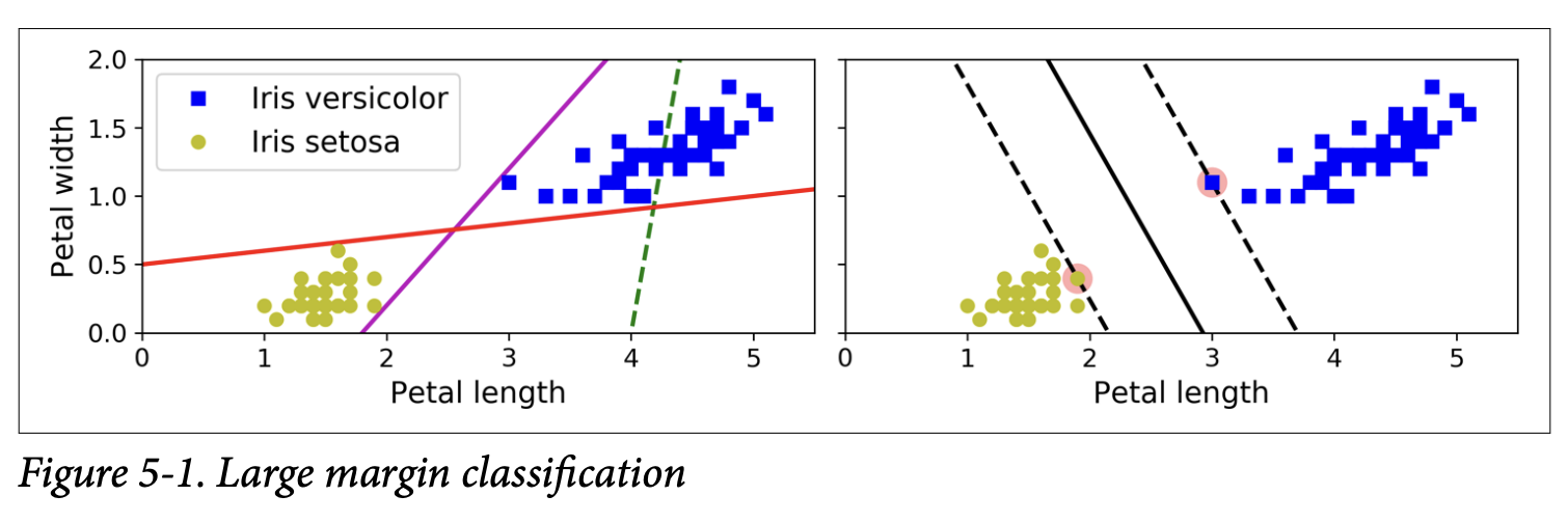
The fundamental idea behind SVMs is best explained with pictures, and Figure 5-1 (page 154) does a great job.

Imagine you have two classes of data points that are linearly separable – meaning you can draw a straight line to separate them perfectly.

• The plot on the left of Figure 5-1 shows three possible straight lines (decision boundaries) that could separate the Iris data.

  • One (dashed) is terrible; it doesn’t even separate the classes.
  • The other two separate the classes perfectly on the training data, but their decision boundaries are very close to some of the training instances. This means they might not generalize well to new, unseen instances. A slight variation in a new point could cause it to be misclassified.

• The plot on the right of Figure 5-1 shows the decision boundary of an SVM classifier.

  • What is it ultimately trying to achieve? An SVM doesn’t just find any line that separates the classes. It tries to find the line that has the largest possible margin between itself and the closest instances from each class.
  • Think of it as fitting the widest possible street between the two classes. The decision boundary is the median line of this street, and the edges of the street are defined by the closest points.
  • This is called large margin classification. The intuition is that a wider margin leads to better generalization because the decision boundary is less sensitive to the exact position of individual training instances and has more “room for error” with new data.

• Support Vectors (Page 154):

  • Notice that the position of this “widest street” is entirely determined by the instances located right on the edge of the street. These instances are called the support vectors (they are circled in Figure 5-1).
  • What they are ultimately trying to achieve: They are the critical data points that “support” or define the decision boundary and the margin. If you move a support vector, the decision boundary will likely change. If you add more training instances that are “off the street” (far away from the margin), they won’t affect the decision boundary at all! The SVM is only sensitive to the points closest to the boundary.

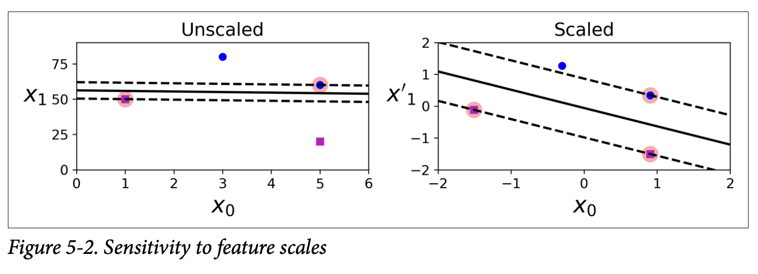
• Sensitivity to Feature Scales (Figure 5-2, page 154):

  

  • The scorpion icon highlights a crucial point: SVMs are sensitive to feature scales.
  • If one feature has a much larger range of values than another (e.g., vertical scale much larger than horizontal in the left plot of Figure 5-2), the “widest street” will tend to be oriented to accommodate the larger scale. The street might look wide in the scaled units, but it might be very narrow along the axis with smaller-scaled features.
  • Solution: Always scale your features (e.g., using Scikit-Learn’s StandardScaler) before training an SVM. The right plot in Figure 5-2 shows a much better, more balanced decision boundary after scaling.
  • What scaling is ultimately trying to achieve: It ensures that all features contribute more equally to the distance calculations involved in finding the largest margin, preventing features with larger numerical values from dominating.

(Page 154-155: Soft Margin Classification)

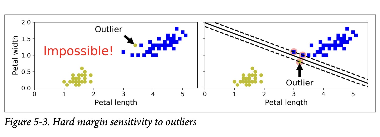
The “widest street” idea so far assumed hard margin classification:

1. All instances must be strictly off the street and on the correct side.
2. This only works if the data is perfectly linearly separable.
3. It’s very sensitive to outliers (Figure 5-3, page 155). A single outlier can make it impossible to find a hard margin, or it can drastically change the decision boundary, leading to poor generalization.

   

To avoid these issues, we use a more flexible approach: Soft Margin Classification.

• What it’s ultimately trying to achieve: Find a good balance between:

  1. Keeping the “street” (margin) as wide as possible.
  2. Limiting margin violations – instances that end up inside the street or even on the wrong side of the decision boundary.

• This allows the model to handle data that isn’t perfectly linearly separable and makes it less sensitive to outliers.

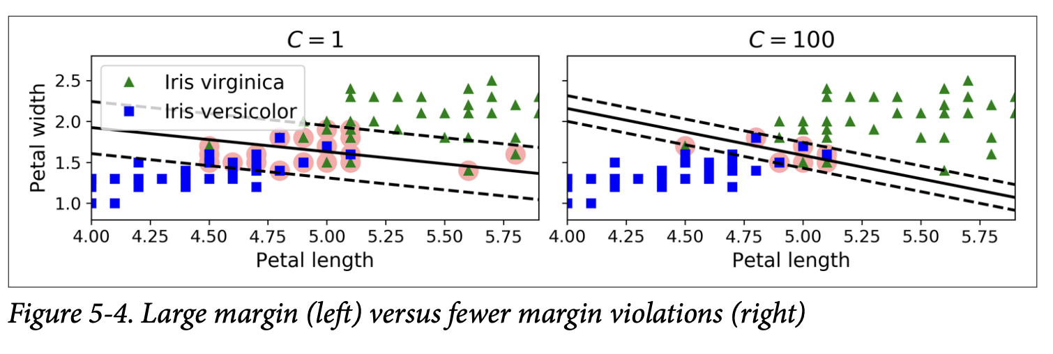
• The C Hyperparameter (Figure 5-4, page 155):

  

  • When using SVMs (e.g., in Scikit-Learn), the hyperparameter C controls this trade-off.
  • Low C value (e.g., C=1 in the left plot of Figure 5-4):
    • Wider street (larger margin).
    • More margin violations are tolerated.
    • This generally leads to a model that is more regularized and might generalize better, even if it makes more mistakes on the training data margin.
  • High C value (e.g., C=100 in the right plot of Figure 5-4):
    • Narrower street (smaller margin).
    • Fewer margin violations are tolerated. The model tries harder to classify all training instances correctly.
    • This can lead to overfitting if C is too high, as the model might be too sensitive to individual data points, including noise or outliers.
  • What C is ultimately trying to achieve: It’s a regularization parameter. A smaller C means more regularization (larger margin, more tolerance for violations). A larger C means less regularization (smaller margin, less tolerance for violations, tries to fit training data more perfectly).
  • If your SVM model is overfitting, try reducing C. If it’s underfitting, try increasing C (but be mindful of also allowing the margin to shrink too much).

• Scikit-Learn Implementation (Page 155-156): The code shows using LinearSVC (Linear Support Vector Classifier) for the Iris dataset: from sklearn.svm import LinearSVC from sklearn.preprocessing import StandardScaler from sklearn.pipeline import Pipeline svm_clf = Pipeline([ ("scaler", StandardScaler()), ("linear_svc", LinearSVC(C=1, loss="hinge")) ]) svm_clf.fit(X, y)

  • Note the use of StandardScaler in a pipeline – good practice!
  • loss="hinge": The hinge loss is the cost function typically associated with linear SVMs (more on this in the “Under the Hood” section).
  • The bird icon (page 156) mentions that unlike Logistic Regression, SVM classifiers generally do not output probabilities directly. They output a decision score, and the sign of the score determines the class.
  • Alternatives for Linear SVMs:
    • SVC(kernel="linear", C=1): Uses the SVC class with a linear kernel. It’s generally slower than LinearSVC but can be useful if you later want to try other kernels.
    • SGDClassifier(loss="hinge", alpha=1/(m*C)): Uses Stochastic Gradient Descent to train a linear SVM. Slower to converge than LinearSVC but good for online learning or very large datasets that don’t fit in memory (out-of-core).
  • The scorpion icon (page 156) gives important tips for LinearSVC:
    • It regularizes the bias term, so centering data (done by StandardScaler) is important.
    • Ensure loss="hinge" is set (not always the default).
    • For better performance, set dual=False unless features > training instances (duality is an advanced optimization concept we’ll touch on).

(Page 157-161: Nonlinear SVM Classification)

Linear SVMs are great, but many datasets aren’t linearly separable. What then?

1. Adding Polynomial Features (Page 157):

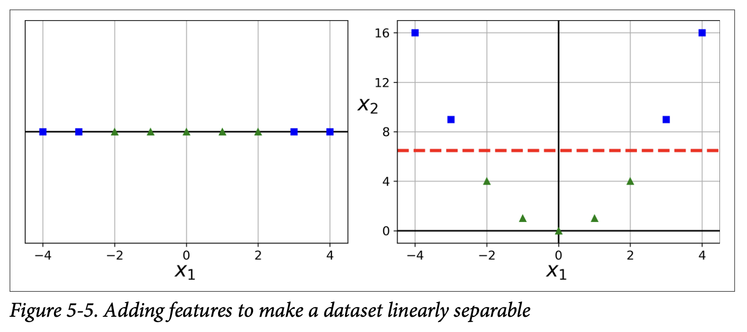
   • As we saw in Chapter 4, you can add polynomial features to your data. This can transform a nonlinearly separable dataset into a linearly separable one in a higher-dimensional space.
   • Figure 5-5 illustrates this: a 1D dataset that’s not linearly separable becomes linearly separable in 2D if you add x₂ = x₁² as a new feature.

     

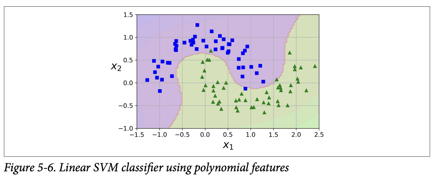
   • Implementation (Moons dataset): from sklearn.datasets import make_moons X, y = make_moons(n_samples=100, noise=0.15) polynomial_svm_clf = Pipeline([ ("poly_features", PolynomialFeatures(degree=3)), ("scaler", StandardScaler()), ("svm_clf", LinearSVC(C=10, loss="hinge")) ]) polynomial_svm_clf.fit(X, y) Figure 5-6 (page 158) shows the resulting decision boundary on the moons dataset. It’s curved and does a decent job!

     

2. The Kernel Trick (Polynomial Kernel - Page 158):

   • Adding polynomial features works, but at high degrees, it creates a huge number of features (combinatorial explosion!), making the model very slow.
   • Enter the Kernel Trick – one of the “magic” ideas in SVMs!
   • What it’s ultimately trying to achieve: It allows you to get the same result as if you had added many polynomial features (even very high-degree ones) without actually creating or adding those features explicitly.
   • This avoids the computational cost and memory overhead of explicitly transforming the data into a very high-dimensional space.
   • How it works (conceptually): Instead of transforming the data points and then taking dot products in the high-dimensional space, the kernel is a function that can compute what the dot product would have been in that high-dimensional space, using only the original low-dimensional data points. (We’ll see more math in “Under the Hood”).
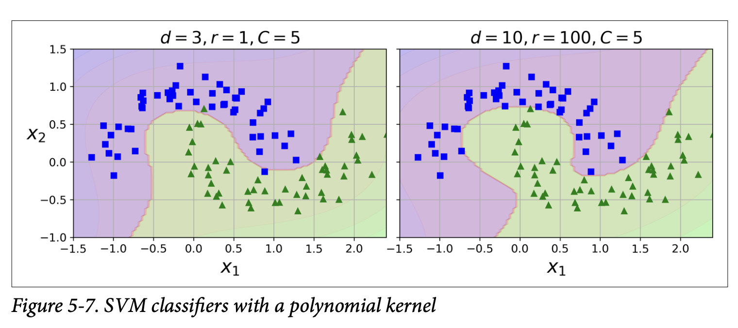
   • Using Polynomial Kernel in Scikit-Learn: from sklearn.svm import SVC poly_kernel_svm_clf = Pipeline([ ("scaler", StandardScaler()), ("svm_clf", SVC(kernel="poly", degree=3, coef0=1, C=5)) ]) poly_kernel_svm_clf.fit(X, y)
     • kernel="poly": Tells SVC to use the polynomial kernel trick.
     • degree=3: Simulates a 3rd-degree polynomial expansion.
     • coef0=1: (Gamma_zero) Controls how much the model is influenced by high-degree vs. low-degree polynomials in the kernel.
     • C=5: Regularization parameter.
     • Figure 5-7 (page 159) shows the results for degree=3 (left) and degree=10 (right). Higher degree can lead to more complex boundaries (and potential overfitting).

       

   • The scorpion icon suggests using grid search to find good hyperparameter values.

3. Similarity Features (Gaussian RBF Kernel - Page 159):

   • Another way to handle nonlinear problems is to add features based on similarity to certain landmarks.
   • Imagine you pick a few landmark points in your feature space. For each data instance, you can calculate how similar it is to each landmark. These similarity scores become new features.
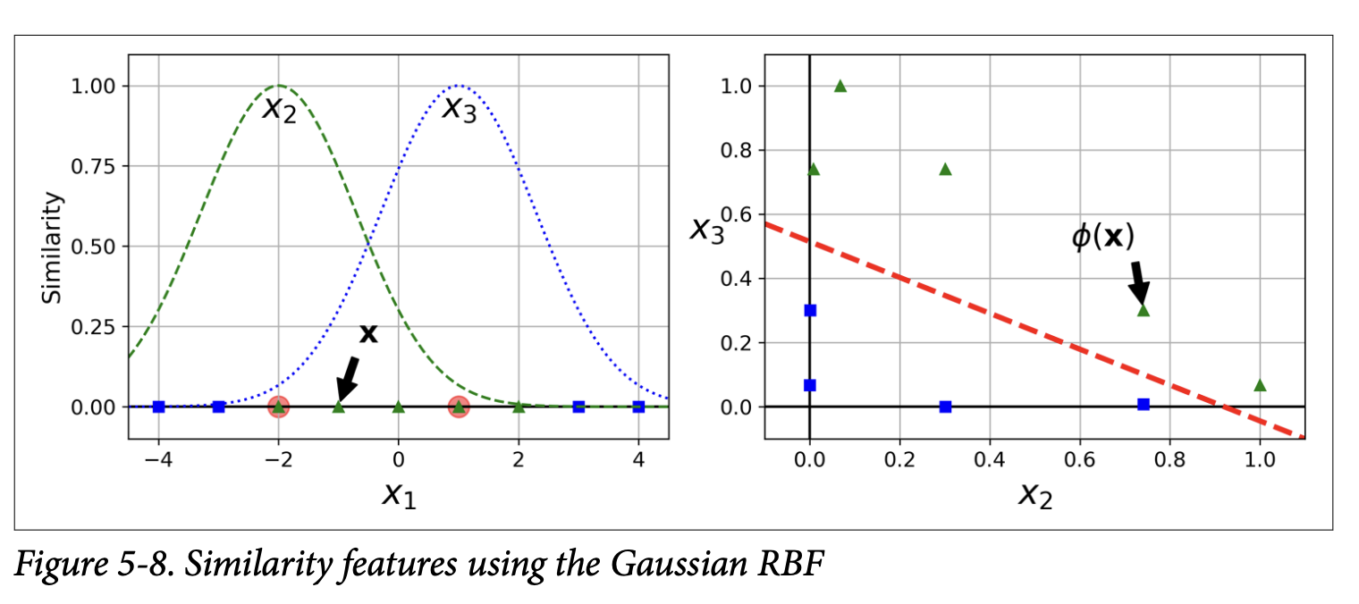
   • Gaussian Radial Basis Function (RBF) as a similarity function (Equation 5-1): φ_γ(x, ℓ) = exp(-γ ||x - ℓ||²)
     • x: An instance.
     • ℓ: A landmark.
     • ||x - ℓ||²: Squared Euclidean distance between the instance and the landmark.
     • γ (gamma): A hyperparameter.
     • What this function is ultimately trying to achieve: It outputs a value between 0 (if x is very far from landmark ℓ) and 1 (if x is at the landmark ℓ). It’s a bell-shaped curve. A higher γ makes the bell narrower (influence of the landmark drops off more quickly).
   • Figure 5-8 shows a 1D dataset. Two landmarks are added. Each original instance x₁ is transformed into two new features: its RBF similarity to landmark 1, and its RBF similarity to landmark 2. The transformed 2D dataset (right plot) becomes linearly separable!

     

   • Choosing landmarks: A simple approach is to create a landmark at the location of every single instance in the dataset. This transforms an m x n dataset into an m x m dataset (if original features are dropped). This can make a dataset linearly separable, but it’s computationally expensive if m is large.

4. Gaussian RBF Kernel (Page 160):

   • Again, the kernel trick comes to the rescue! The Gaussian RBF kernel allows SVMs to get the same effect as adding many RBF similarity features, without actually computing them.
   • Using Gaussian RBF Kernel in Scikit-Learn: rbf_kernel_svm_clf = Pipeline([ ("scaler", StandardScaler()), ("svm_clf", SVC(kernel="rbf", gamma=5, C=0.001)) ]) rbf_kernel_svm_clf.fit(X, y)
     • kernel="rbf": Use the Gaussian RBF kernel.
     • gamma (γ): Controls the width of the RBF “bell.”
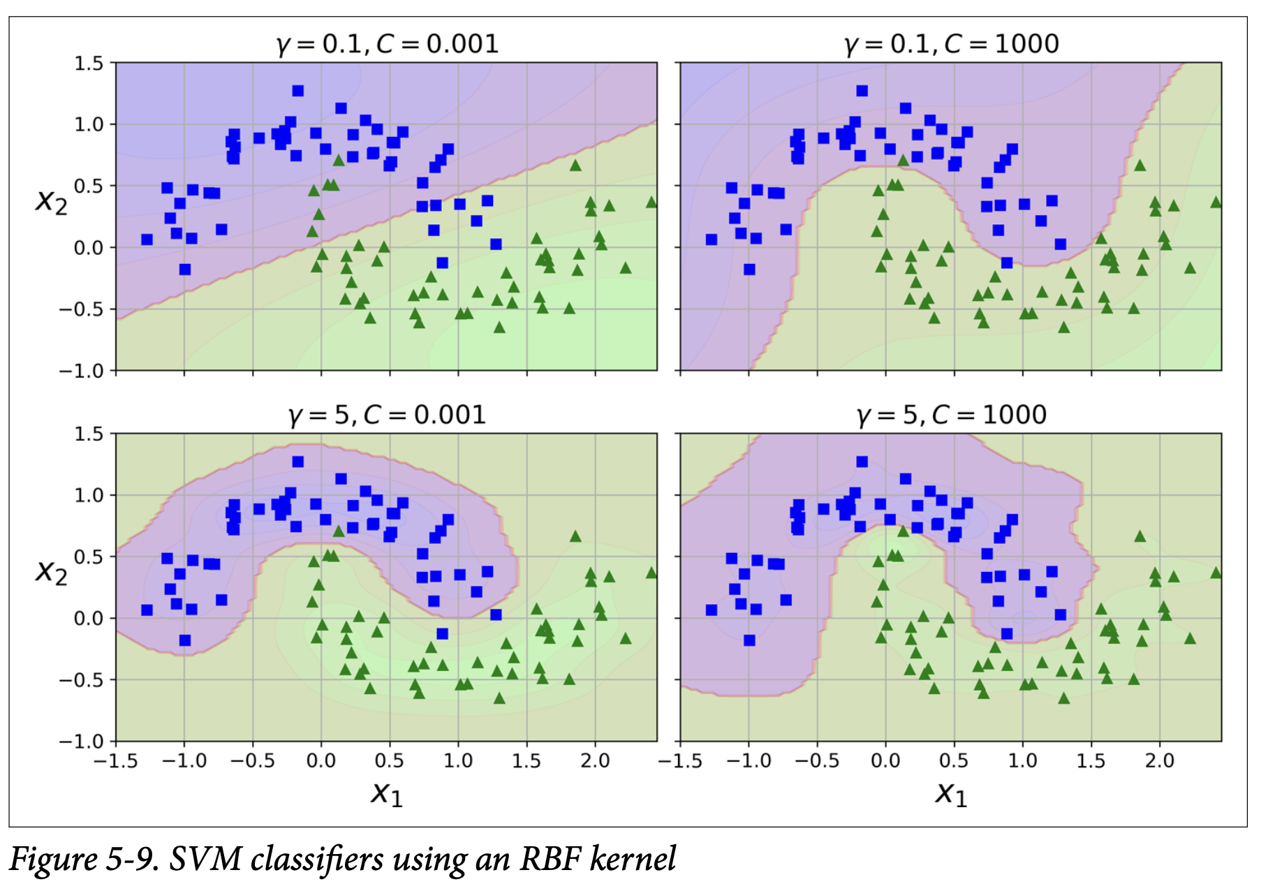
       • Increasing gamma: Makes the bell narrower. Each instance’s range of influence is smaller. Decision boundary becomes more irregular, wiggling around individual instances (can lead to overfitting). (See Figure 5-9, page 161, comparing gamma=0.1 to gamma=5).
       • Decreasing gamma: Makes the bell wider. Instances have a larger range of influence. Decision boundary becomes smoother (can lead to underfitting if too smooth).
       • So, gamma acts like a regularization hyperparameter: if overfitting, reduce gamma; if underfitting, increase gamma.
     • C: Regularization parameter, as before. Lower C = more regularization.
     • Figure 5-9 shows how different gamma and C values affect the decision boundary for the RBF kernel.

       

   • Which kernel to use? (Scorpion icon, page 161):
     • Always try linear kernel first (LinearSVC is much faster than SVC(kernel="linear")). Especially if training set is large or has many features.
     • If training set isn’t too large, try Gaussian RBF kernel next. It works well in most cases.
     • If you have time/compute power, experiment with other kernels (e.g., polynomial, or specialized kernels like string kernels for text) using cross-validation and grid search.

(Page 162: Computational Complexity)

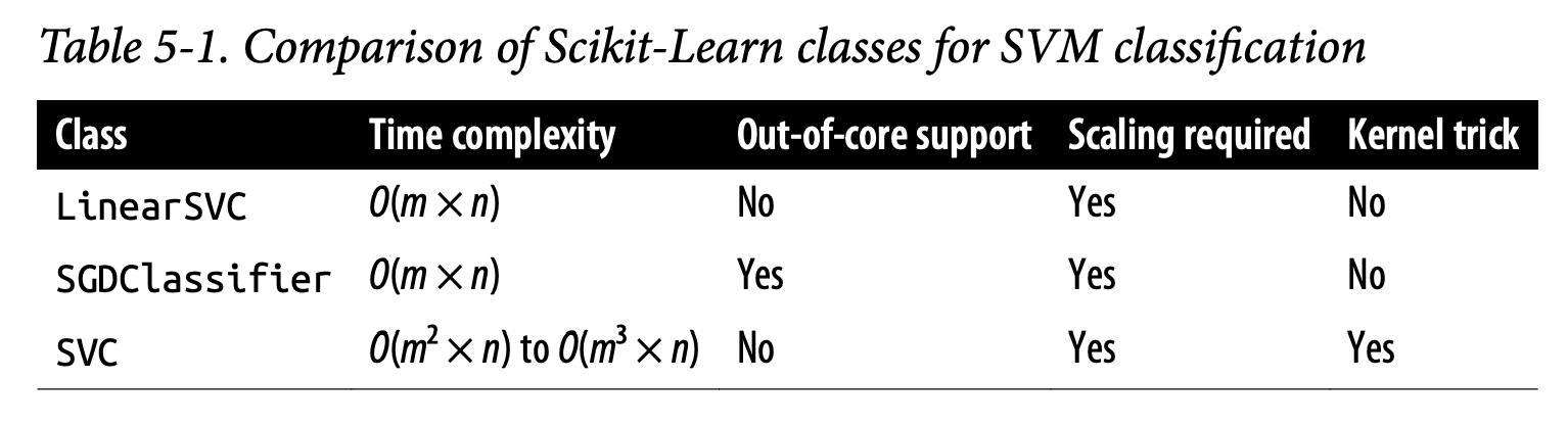
• LinearSVC: Based on liblinear. Does not support the kernel trick. Scales almost linearly with number of instances (m) and features (n) – roughly O(m × n). Good for large datasets if a linear model is sufficient.
• SVC: Based on libsvm. Does support the kernel trick.
  • Training time complexity: Between O(m² × n) and O(m³ × n).
  • Gets dreadfully slow when m (number of instances) is large (e.g., hundreds of thousands).
  • Perfect for complex small or medium-sized datasets.
  • Scales well with number of features, especially sparse features.
• Table 5-1 summarizes this.

  

(Page 162-163: SVM Regression)

SVMs can also do regression!

• The Goal (Reversed Objective):
  • For classification: Fit the widest street between classes, limiting margin violations.
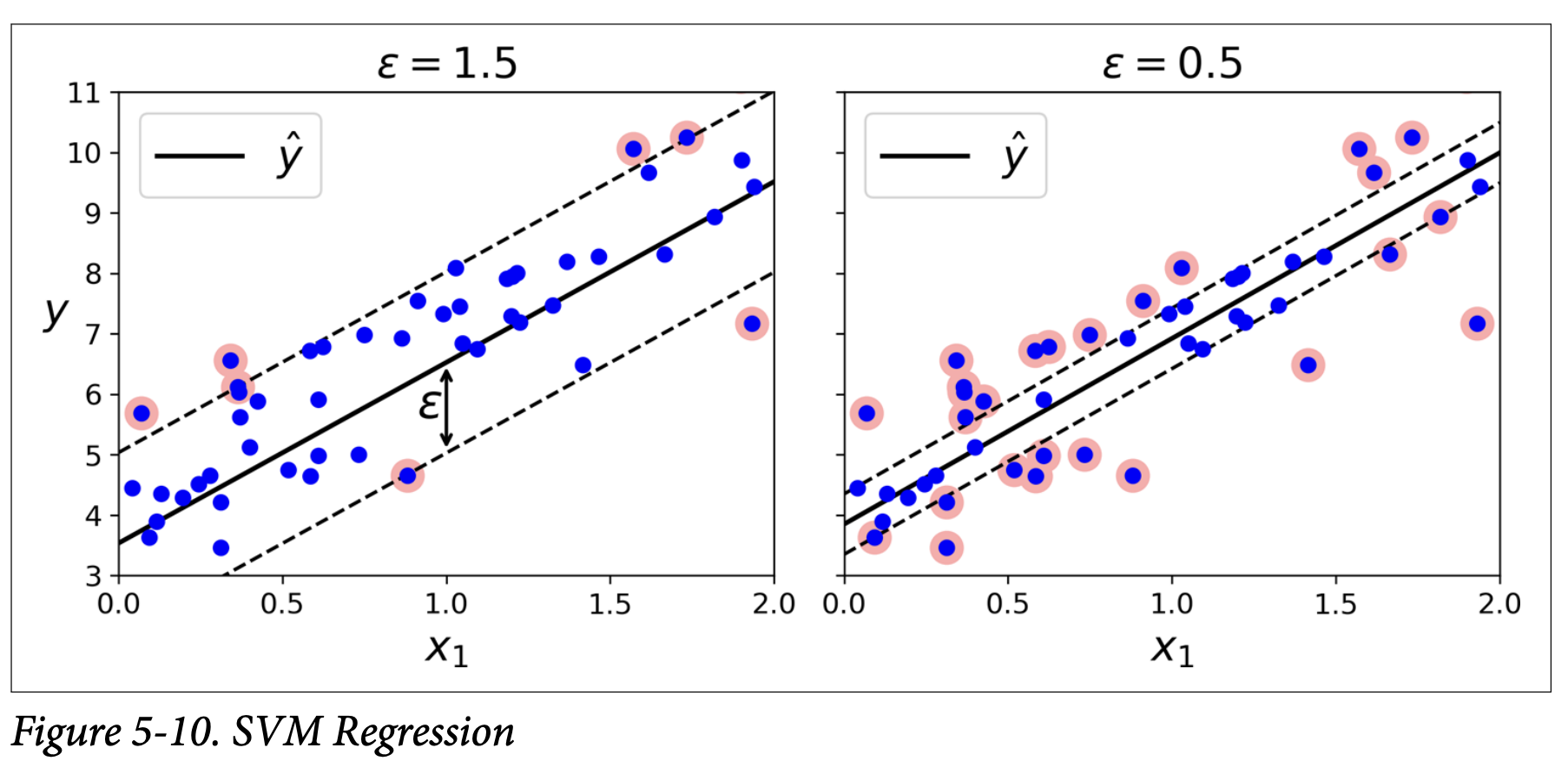
  • For SVM Regression (SVR): Fit as many instances as possible on the street, while limiting margin violations (instances off the street).
• ϵ (epsilon) hyperparameter: Controls the width of the street. (Figure 5-10, page 163).

  

  • Larger ϵ: Wider street. More instances can fit inside the margin without penalty.
  • Smaller ϵ: Narrower street.
• ϵ-insensitive: Adding more training instances within the margin (inside the street) does not affect the model’s predictions.
• Scikit-Learn Classes:
  • LinearSVR: For linear SVM regression. from sklearn.svm import LinearSVR svm_reg = LinearSVR(epsilon=1.5) (Data should be scaled and centered first).
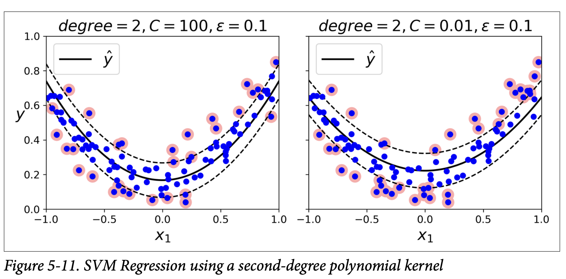
  • SVR: For nonlinear SVM regression using kernels. from sklearn.svm import SVR svm_poly_reg = SVR(kernel="poly", degree=2, C=100, epsilon=0.1) Figure 5-11 (page 164) shows SVR with a polynomial kernel.

    

    • Large C: Little regularization. Model tries to fit data points closely.
    • Small C: More regularization. Smoother fit.
• LinearSVR scales linearly with training set size. SVR gets slow as training set size grows (like SVC).
• SVMs can also be used for outlier detection.

Under the hood

Let’s start with the big picture goals for a Linear SVM:

Goal 1: Separate the Classes. (Obvious) We want a line (or plane/hyperplane) that divides the data.

Goal 2: Make this Separation as “Safe” or “Robust” as Possible (Large Margin). This is the core SVM idea. We don’t just want any separating line; we want the one that stays farthest away from the closest points of both classes. This “widest street” (the margin) makes the classifier less sensitive to small variations in data and hopefully better at classifying new, unseen points.

How do we achieve Goal 2 mathematically? (This is where w and b come in)

1. The Decision Boundary: Our line is defined by wᵀx + b = 0.

   • w (weights vector): Determines the orientation or slope of the line.
   • b (bias): Shifts the line up or down without changing its orientation.

2. The “Street”: The edges of our street (the margins) are defined by wᵀx + b = 1 and wᵀx + b = -1.

   • All positive class points should ideally be on or “above” wᵀx + b = 1.
   • All negative class points should ideally be on or “below” wᵀx + b = -1.

3. Width of the Street: It turns out mathematically that the width of this street is 2 / ||w|| (where ||w|| is the magnitude or length of the vector w).

   • Key Insight: To make the street (margin) WIDE, we need ||w|| to be SMALL.
   • What are we trying to achieve by minimizing ||w||? We are trying to maximize the margin.
   • For mathematical convenience (easier to take derivatives), instead of minimizing ||w||, we minimize (1/2)||w||² (which is (1/2)wᵀw). Minimizing one also minimizes the other.

So, the Training Objective (Hard Margin - Equation 5-3) becomes:

• Objective: Minimize (1/2)wᵀw (make the margin large)
• Subject to (Constraints): t⁽ⁱ⁾(wᵀx⁽ⁱ⁾ + b) ≥ 1 for all training instances i.
  • t⁽ⁱ⁾ is +1 for positive class, -1 for negative.
  • This constraint says: “Every training point must be on the correct side of its respective margin boundary, or right on it.”

What this constrained optimization is ultimately trying to achieve: Find the line orientation (w) and position (b) that gives the widest possible street while ensuring all training points are correctly classified and stay out of (or on the edge of) the street.

What if the data isn’t perfectly separable (Soft Margin - Equation 5-4)?

Real data is messy. Outliers exist. We might not be able to find a street where all points are perfectly on the correct side.

• Slack Variables ζ⁽ⁱ⁾ (zeta): We introduce a “fudge factor” or “slack” ζ⁽ⁱ⁾ ≥ 0 for each point i.
  • If ζ⁽ⁱ⁾ = 0, point i respects the margin.
  • If ζ⁽ⁱ⁾ > 0, point i violates the margin (it’s inside the street or on the wrong side). The value of ζ⁽ⁱ⁾ tells us how much it violates.
• New Objective (Soft Margin):
  • Minimize (1/2)wᵀw + C Σᵢ ζ⁽ⁱ⁾
  • Subject to: t⁽ⁱ⁾(wᵀx⁽ⁱ⁾ + b) ≥ 1 - ζ⁽ⁱ⁾ and ζ⁽ⁱ⁾ ≥ 0.
• What this soft margin optimization is ultimately trying to achieve:
  1. Still try to make (1/2)wᵀw small (maximize margin).
  2. But also try to make Σᵢ ζ⁽ⁱ⁾ small (minimize the total amount of margin violations).
  3. The hyperparameter C is the trade-off.
     • Large C: Penalizes violations heavily. Model will try very hard to get points right, even if it means a narrower margin. (Closer to hard margin).
     • Small C: Tolerates more violations in favor of a wider margin. (More regularization).

The hard margin and soft margin problems are both convex quadratic optimization problems with linear constraints. This problem (finding w, b, and ζs) is a Quadratic Programming (QP) problem. We can give it to a standard QP solver.

Why Introduce the “Dual Problem” (Equation 5-6)? This is often the confusing part.

Solving the QP problem directly (called the “primal problem”) is fine for linear SVMs. But it has limitations:

1. It can be slow if the number of features n is very large.
2. More importantly, it doesn’t allow for the “kernel trick” which is essential for efficient non-linear SVMs.

The Dual Problem is a different but related mathematical formulation of the same optimization task.

• Instead of finding w and b directly, it focuses on finding a set of new variables, αᵢ (alpha-i), one for each training instance.
• Key Property of these αᵢs: It turns out that αᵢ will be greater than zero only for the support vectors. For all other data points, αᵢ will be zero!
• What solving the dual problem is ultimately trying to achieve: It’s finding the importance (αᵢ) of each training instance in defining the optimal margin. Only the support vectors end up having non-zero importance.

Why is the Dual useful?

1. Computational Efficiency in some cases: If the number of training instances m is smaller than the number of features n, solving the dual can be faster.
2. THE KERNEL TRICK (THIS IS THE BIG ONE!): Look at the dual objective function (Equation 5-6): minimize (1/2) Σᵢ Σⱼ αᵢαⱼt⁽ⁱ⁾t⁽ʲ⁾(x⁽ⁱ⁾ᵀx⁽ʲ⁾) - Σᵢ αᵢ Notice the term (x⁽ⁱ⁾ᵀx⁽ʲ⁾). This is a dot product between pairs of training instances. The solution w from the dual (Equation 5-7) also involves sums of αᵢt⁽ⁱ⁾x⁽ⁱ⁾. And crucially, when you make predictions using the dual formulation (Equation 5-11), the decision function becomes: h(x_new) = Σᵢ αᵢt⁽ⁱ⁾(x⁽ⁱ⁾ᵀx_new) + b (sum over support vectors i) Again, it only involves dot products between the support vectors and the new instance x_new.

The Kernel Trick - The “Aha!” Moment for Nonlinear SVMs:

Now, imagine we want to do nonlinear classification. One way (as discussed for Polynomial Regression) is to map our data x to a much higher-dimensional space using a transformation φ(x), where the data becomes linearly separable.

• If we did this explicitly, we would then have to compute dot products like φ(x⁽ⁱ⁾)ᵀφ(x⁽ʲ⁾) in this very high (maybe even infinite) dimensional space. This would be computationally impossible or extremely inefficient.

• The Kernel Trick says: What if there’s a special function K(a,b) called a kernel that can compute the dot product φ(a)ᵀφ(b) for us, using only the original vectors a and b, without us ever having to compute φ(a) or φ(b) explicitly?

  • For example, the polynomial kernel K(a,b) = (γaᵀb + r)ᵈ calculates what the dot product would be if you mapped a and b to a d-th degree polynomial feature space.
  • The Gaussian RBF kernel K(a,b) = exp(-γ ||a - b||²) implicitly maps to an infinite-dimensional space!

• What the kernel trick is ultimately trying to achieve: It allows us to get the benefit of working in a very high-dimensional feature space (where complex separations might become linear) without the prohibitive computational cost of actually creating and working with those high-dimensional vectors. We just replace all dot products x⁽ⁱ⁾ᵀx⁽ʲ⁾ in the dual formulation and in the prediction equation with K(x⁽ⁱ⁾, x⁽ʲ⁾).

So, the “Under the Hood” Flow for Kernelized SVMs:

1. Start with a nonlinear problem.
2. Choose a kernel function K(a,b) (e.g., Polynomial, RBF). This implicitly defines a transformation φ to a higher-dimensional space where the data is hopefully linearly separable.
3. Solve the DUAL optimization problem (Equation 5-6, but with x⁽ⁱ⁾ᵀx⁽ʲ⁾ replaced by K(x⁽ⁱ⁾, x⁽ʲ⁾)). This finds the αᵢ values (which will be non-zero only for support vectors).
   • What this is trying to achieve: Find the “importance” of each training point in defining the optimal linear margin in that implicit high-dimensional space.
4. Make predictions for a new instance x_new (Equation 5-11, with K): h(x_new) = Σᵢ αᵢt⁽ⁱ⁾K(x⁽ⁱ⁾, x_new) + b
   • What this is trying to achieve: Classify the new point based on its kernel “similarity” (as defined by K) to the support vectors, effectively performing a linear separation in the implicit high-dimensional space.

Think of it like this:

• Primal problem (for linear SVM): Directly find the best “street” (w, b) in the original feature space.
• Dual problem (for linear SVM): Find out which data points (αᵢ > 0) are the crucial “support posts” for that street. This formulation happens to only use dot products.
• Kernelized SVM (using the dual): We want a curvy street in our original space. The kernel trick lets us pretend we’ve straightened out the data into a super high-dimensional space where a straight street works. We use the dual formulation because it only relies on dot products, and we can replace those dot products with our kernel function K. The kernel function cleverly calculates what those dot products would have been in the high-dimensional space, without us ever going there.

So, the progression of “what are we trying to achieve”:

1. Linear SVM (Primal): Maximize margin directly by finding w and b.
2. Challenges: Can be slow for many features, doesn’t easily extend to non-linear.
3. Linear SVM (Dual): Reformulate to find αs (support vector indicators). Only uses dot products.
4. Kernel Trick Motivation: We want non-linear separation. Idea: map to a higher space where it’s linear. Problem: mapping is expensive.
5. Kernelized SVM (Dual + Kernel): Realize the dual only needs dot products. If we can find a kernel K(a,b) that equals φ(a)ᵀφ(b) without computing φ, we can do complex non-linear classification efficiently by solving the dual problem with K and making predictions with K.

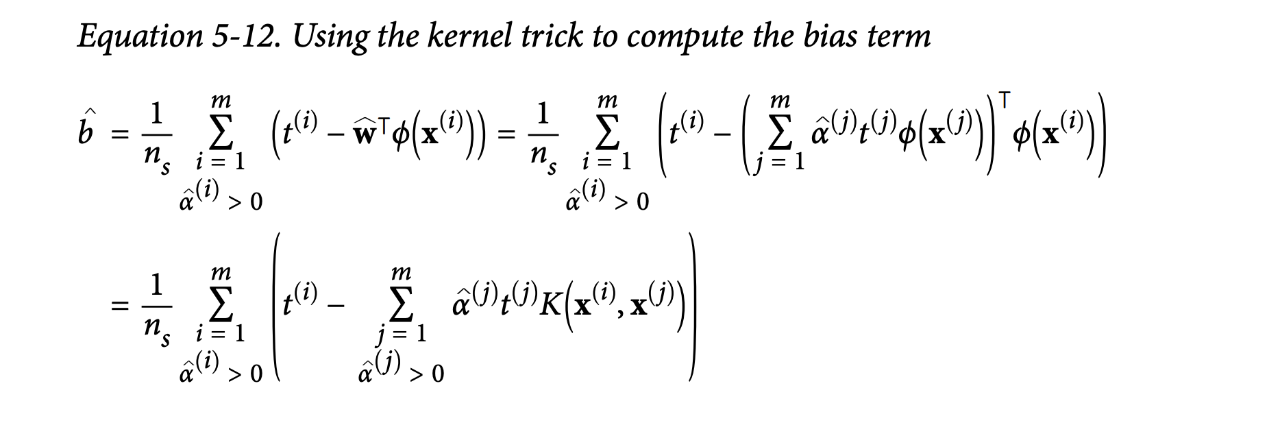
The “headache” the book mentions with Equation 5-12 for computing b with kernels is because even b needs to be calculated using these kernelized dot products, as we no longer have an explicit w in the original space.

It’s a chain of clever mathematical steps, each designed to overcome a limitation of the previous one, ultimately allowing us to achieve large margin classification for complex, non-linear data in an efficient way. The dual formulation is the bridge that makes the kernel trick possible.

Does this step-by-step focus on the “why” for each part (especially the dual and kernel) help make the overall strategy a bit more intuitive? It’s okay if it still feels complex; SVM theory is one of the more mathematically rich areas in classical ML.

---

Glossary

(Page 164-173: Under the Hood - How SVMs Work)

This is where the math gets a bit deeper, but remember our goal: “what is it ultimately trying to achieve?” The book changes notation here for SVMs, which is common:

• Bias term: b (instead of θ₀)

• Feature weights vector: w (instead of θ₁ to θₙ)

• No x₀=1 bias input feature is added.

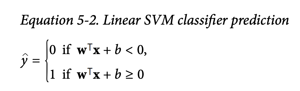
• Decision Function and Predictions (Linear SVM - page 165):

  • Decision function: wᵀx + b
  • Equation 5-2: Linear SVM classifier prediction

    

    ŷ = 1 if wᵀx + b ≥ 0 ŷ = 0 if wᵀx + b < 0 (or class -1 if using -1/1 labels)
  • Figure 5-12 shows this in 3D for 2 features: wᵀx + b is a plane. The decision boundary is where wᵀx + b = 0 (a line). The “street” is defined by wᵀx + b = 1 and wᵀx + b = -1. These are parallel lines/planes forming the margin.

    

• Training Objective (Page 166):

  • Goal: Find w and b that make the margin (the “street”) as wide as possible, while controlling margin violations.

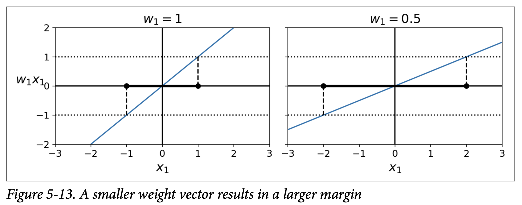
  • The slope of the decision function is ||w|| (norm of the weight vector).

  • Key insight (Figure 5-13): The smaller the norm ||w||, the larger the margin. (If you divide w and b by 2, the slope ||w||/2 is halved, effectively doubling the distance to the ±1 lines, thus doubling the margin width).

    

  • So, we want to minimize ||w|| (or equivalently, minimize (1/2)wᵀw which is (1/2)||w||² – easier to differentiate).

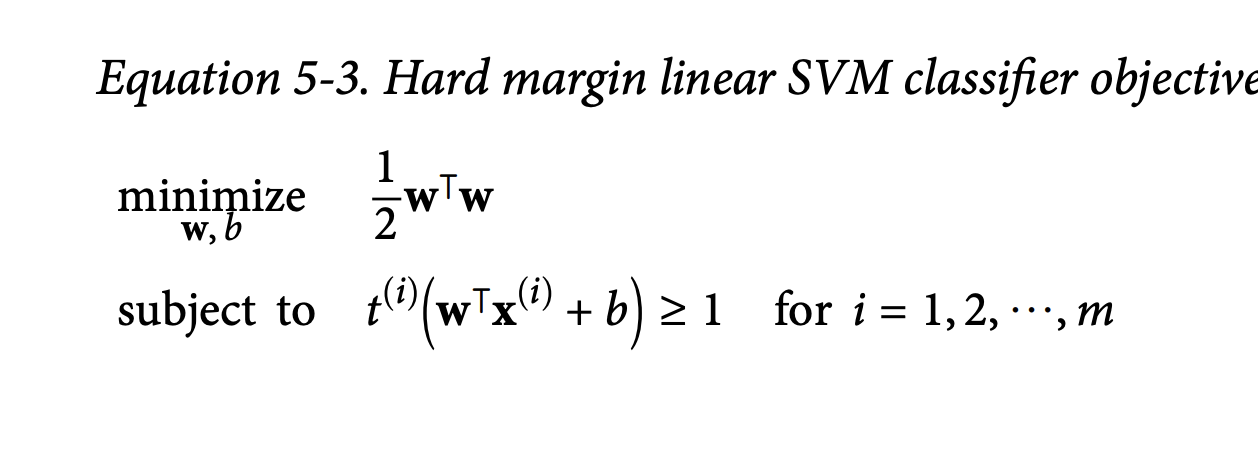
  • Hard Margin Objective (Equation 5-3):

    

    minimize (1/2)wᵀw subject to t⁽ⁱ⁾(wᵀx⁽ⁱ⁾ + b) ≥ 1 for all instances i.
    • t⁽ⁱ⁾ is 1 for positive class, -1 for negative class.
    • The constraint t⁽ⁱ⁾(wᵀx⁽ⁱ⁾ + b) ≥ 1 means:
      • For positive instances (t⁽ⁱ⁾=1): wᵀx⁽ⁱ⁾ + b ≥ 1 (on or outside the positive margin boundary).
      • For negative instances (t⁽ⁱ⁾=-1): wᵀx⁽ⁱ⁾ + b ≤ -1 (on or outside the negative margin boundary).
    • What it’s ultimately trying to achieve: Find the w with the smallest norm (largest margin) such that all points are correctly classified and outside or on the margin boundaries.

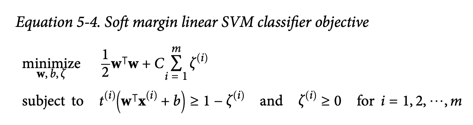
  • Soft Margin Objective (Equation 5-4, page 167):

    

    To allow for margin violations, introduce slack variables ζ⁽ⁱ⁾ ≥ 0 (zeta-i) for each instance i. ζ⁽ⁱ⁾ measures how much instance i is allowed to violate the margin. minimize (1/2)wᵀw + C Σᵢ ζ⁽ⁱ⁾ subject to t⁽ⁱ⁾(wᵀx⁽ⁱ⁾ + b) ≥ 1 - ζ⁽ⁱ⁾ and ζ⁽ⁱ⁾ ≥ 0.
    • What it’s ultimately trying to achieve:
      • Still minimize (1/2)wᵀw (maximize margin).
      • But also minimize Σᵢ ζ⁽ⁱ⁾ (sum of slack/violations).
      • C is the hyperparameter that trades off between these two conflicting objectives: large margin vs. few violations.
        • Small C: Margin width is prioritized (more slack allowed).
        • Large C: Few violations prioritized (margin might be smaller).

• Quadratic Programming (QP) (Page 167):

  • Both hard and soft margin SVM objectives are convex quadratic optimization problems with linear constraints. These are known as QP problems.
  • Specialized QP solvers exist to find the optimal w and b. Equation 5-5 gives the general QP formulation. The book explains how to map SVM parameters to this general form.

• The Dual Problem (Page 168-169):

  • For constrained optimization problems (like SVMs), there’s often a “primal problem” and a related “dual problem.”
  • Solving the dual can sometimes be easier or offer advantages. For SVMs, the dual problem:
    • Is faster to solve than the primal when number of training instances (m) < number of features (n).
    • Crucially, makes the kernel trick possible! (The primal does not).
  • Equation 5-6: Dual form of the linear SVM objective:

    

    This involves minimizing a function with respect to new variables αᵢ (alpha-i), one for each training instance. minimize (1/2) Σᵢ Σⱼ αᵢαⱼt⁽ⁱ⁾t⁽ʲ⁾(x⁽ⁱ⁾ᵀx⁽ʲ⁾) - Σᵢ αᵢ subject to αᵢ ≥ 0.
  • Once you find the optimal α̂ vector (using a QP solver), you can compute ŵ and b̂ for the primal problem using Equation 5-7.
  • An important property is that αᵢ will be non-zero only for the support vectors! Most αᵢ will be zero.

• Kernelized SVMs (The Kernel Trick Explained - Page 169-171): This is where the magic happens for nonlinear SVMs.

  • Suppose we have a mapping function φ(x) that transforms our input x into a higher-dimensional space where it might become linearly separable (Equation 5-8 for a 2nd-degree polynomial mapping).
  • If we apply this transformation φ to all training instances, the dual problem (Equation 5-6) would contain dot products of these transformed vectors: φ(x⁽ⁱ⁾)ᵀφ(x⁽ʲ⁾).
  • The Key Insight (Equation 5-9 for 2nd-degree polynomial): It turns out that for some transformations φ, the dot product φ(a)ᵀφ(b) in the high-dimensional space can be computed by a simpler function K(a,b) using only the original vectors a and b. For the 2nd-degree polynomial mapping, φ(a)ᵀφ(b) = (aᵀb)².
  • The Kernel Function K(a,b): A kernel K(a,b) is a function that computes φ(a)ᵀφ(b) based only on a and b, without needing to know or compute φ itself!
    • What it’s ultimately trying to achieve: It allows us to operate in a very high (even infinite) dimensional feature space implicitly, without ever actually creating those features. This avoids the computational nightmare of explicit transformation.
  • So, in the dual problem (Equation 5-6), we just replace x⁽ⁱ⁾ᵀx⁽ʲ⁾ with K(x⁽ⁱ⁾, x⁽ʲ⁾).
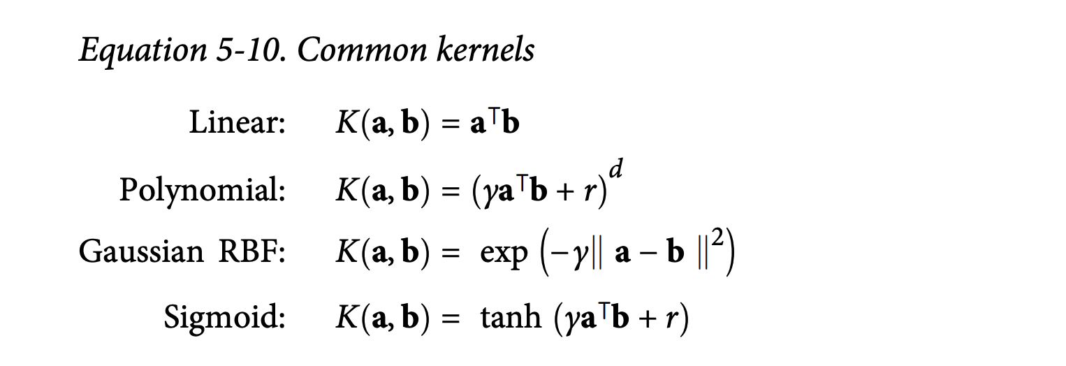
  • Common Kernels (Equation 5-10, page 171):

    

    • Linear: K(a,b) = aᵀb (no transformation)
    • Polynomial: K(a,b) = (γaᵀb + r)ᵈ
    • Gaussian RBF: K(a,b) = exp(-γ ||a - b||²)
    • Sigmoid: K(a,b) = tanh(γaᵀb + r)
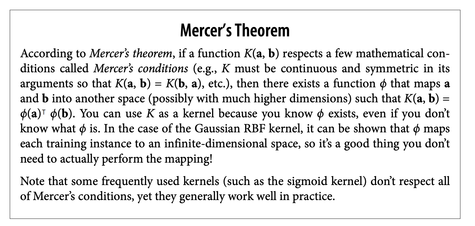
  • Mercer’s Theorem (sidebar): Provides mathematical conditions for a function K to be a valid kernel (i.e., for a corresponding φ to exist). Gaussian RBF kernel actually maps to an infinite-dimensional space! Good thing we don’t have to compute φ.

    

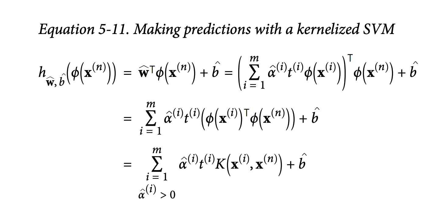
• Making Predictions with Kernels (Equation 5-11, page 172):

  

  We need w to make predictions, but w lives in the (potentially huge) φ space. How do we predict without computing w? Equation 5-7 for w involves φ(x⁽ⁱ⁾). If we plug this into the decision function wᵀφ(x⁽ⁿ⁾) + b, we get an equation that only involves dot products of φ terms, which can be replaced by kernels: h(x⁽ⁿ⁾) = Σᵢ αᵢt⁽ⁱ⁾K(x⁽ⁱ⁾, x⁽ⁿ⁾) + b (sum over support vectors i where αᵢ > 0).
  • What it’s ultimately trying to achieve: Predictions for a new instance x⁽ⁿ⁾ are made by computing its kernel similarity to only the support vectors.
  • The bias term b can also be computed using kernels (Equation 5-12).

    

• Online SVMs (Page 172-173): For online learning (incremental learning).

  • One method for linear SVMs: Use Gradient Descent on a cost function derived from the primal problem (Equation 5-13).
  • Equation 5-13: Linear SVM classifier cost function (Hinge Loss) J(w,b) = (1/2)wᵀw + C Σᵢ max(0, 1 - t⁽ⁱ⁾(wᵀx⁽ⁱ⁾ + b))
    • (1/2)wᵀw: Aims for a large margin (small w).
    • max(0, 1 - t⁽ⁱ⁾(wᵀx⁽ⁱ⁾ + b)): This is the hinge loss.
      • What hinge loss is ultimately trying to achieve: It penalizes instances that violate the margin. If an instance i is correctly classified and outside or on the margin (t⁽ⁱ⁾(wᵀx⁽ⁱ⁾ + b) ≥ 1), then 1 - t⁽ⁱ⁾(...) ≤ 0, so max(0, ...) = 0 (zero loss for this instance).
      • If it violates the margin, the loss is proportional to how far it is from its correct margin boundary.
    • This cost function is what SGDClassifier(loss="hinge") minimizes.
  • Online kernelized SVMs are also possible but more complex.

And that’s the grand tour of Support Vector Machines! The core idea of large margin classification is simple and elegant. The kernel trick is the “magic” that allows SVMs to handle complex nonlinear data efficiently by implicitly operating in very high-dimensional feature spaces.

The “Under the Hood” section is definitely more mathematical, but hopefully, by focusing on “what is it ultimately trying to achieve” for each equation (like minimizing ||w|| for a large margin, or using kernels to avoid explicit high-dimensional transformations), the core concepts become clearer.

Any part of that, especially the kernel trick or the dual problem, that still feels a bit fuzzy?