Introduction to Decision Trees

Alright class, settle in! After exploring the world of Support Vector Machines, we’re now turning our attention to another incredibly versatile and powerful family of algorithms: Decision Trees.

• Versatility: Like SVMs, Decision Trees can perform both classification and regression tasks. They can even handle multioutput tasks (where each instance can have multiple output labels or values).
• Power: They are capable of fitting complex datasets. You might recall from Chapter 2, when we looked at the California housing data, a DecisionTreeRegressor was able to fit the training data perfectly (though, as we noted, it was actually overfitting).
• Fundamental Building Blocks: Decision Trees are also the core components of Random Forests (which we’ll see in Chapter 7). Random Forests are among the most powerful and widely used ML algorithms today. So, understanding Decision Trees is crucial for understanding Random Forests.

What this chapter will cover:

1. How to train, visualize, and make predictions with Decision Trees.
2. The CART (Classification and Regression Tree) training algorithm, which Scikit-Learn uses.
3. How to regularize Decision Trees (to prevent overfitting).
4. How they’re used for regression tasks.
5. Some of their limitations.

(Page 175-176: Training and Visualizing a Decision Tree)

Let’s start by building one to see how it works. We’ll use the Iris dataset (which we’ve seen before, for example, with Logistic Regression in Chapter 4).

• The Code: from sklearn.datasets import load_iris from sklearn.tree import DecisionTreeClassifier

  iris = load_iris() X = iris.data[:, 2:] # petal length and width only y = iris.target # species (0: setosa, 1: versicolor, 2: virginica)

  tree_clf = DecisionTreeClassifier(max_depth=2) tree_clf.fit(X, y)

  • We’re only using two features: petal length and petal width, to make it easy to visualize.
  • max_depth=2: This is a crucial hyperparameter. We are telling the tree not to grow beyond a depth of 2 levels. This is a form of regularization to prevent it from becoming too complex and overfitting. If we didn’t set this, the tree might grow very deep to try and perfectly classify every single training instance.

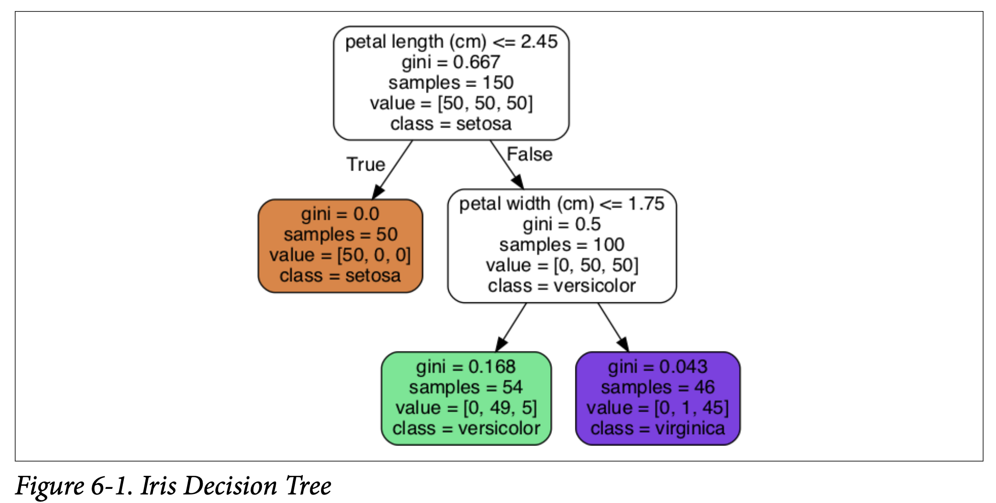
• Visualizing the Tree (Page 176): One of the great things about Decision Trees is that they are very intuitive and easy to visualize. Scikit-Learn provides a function export_graphviz to help with this. from sklearn.tree import export_graphviz export_graphviz( tree_clf, out_file="iris_tree.dot", feature_names=iris.feature_names[2:], class_names=iris.target_names, rounded=True, filled=True ) This creates a .dot file. You then use the dot command-line tool (from the Graphviz package, which you’d need to install separately) to convert this into an image, like a PNG: $ dot -Tpng iris_tree.dot -o iris_tree.png

  Figure 6-1 (Iris Decision Tree): This is the visual representation of our trained tree. It’s a flowchart-like structure. Let’s understand its components:

  

  • Nodes: Each box is a node.
    • Root Node (Depth 0, at the top): This is where you start. It asks a question about a feature. In Figure 6-1, it asks: “petal length (cm) <= 2.45?”
    • Child Nodes: Based on the answer (True or False), you move to a child node.
    • Leaf Nodes: Nodes that don’t have any children. These nodes make the final prediction.
  • Information in each node:
    • Question/Condition: E.g., “petal length (cm) <= 2.45”.
    • gini: This measures the impurity of the node. We’ll discuss this more soon. A gini score of 0 means the node is “pure” – all training instances that reach this node belong to the same class.
    • samples: How many training instances from the dataset fall into this node.
    • value: How many training instances of each class fall into this node. For example, value = [50, 50, 50] at the root means there were 50 Setosa, 50 Versicolor, and 50 Virginica instances in the training set that reached this node (which is all of them initially).
    • class: The class that would be predicted if this node were a leaf node (i.e., the majority class among the samples in this node).

(Page 176-177: Making Predictions)

How do you use this tree (Figure 6-1) to classify a new iris flower? It’s like a game of “20 Questions.”

1. Start at the root node (depth 0).
   • Question: Is the flower’s petal length ≤ 2.45 cm?
2. If YES (True): Move to the left child node (depth 1, left).
   • This node in Figure 6-1 has gini = 0.0, samples = 50, value = [50, 0, 0], class = setosa.
   • This is a leaf node (it has no further questions/children).
   • So, the prediction is Iris setosa.
3. If NO (False, meaning petal length > 2.45 cm): Move to the right child node (depth 1, right).
   • This node is not a leaf node. It asks another question.
   • Question: Is the flower’s petal width ≤ 1.75 cm?
4. If YES (True, petal length > 2.45 cm AND petal width ≤ 1.75 cm): Move to this node’s left child (depth 2, middle of bottom row).
   • This is a leaf node. class = versicolor.
   • Prediction: Iris versicolor.
5. If NO (False, petal length > 2.45 cm AND petal width > 1.75 cm): Move to this node’s right child (depth 2, rightmost bottom row).
   • This is a leaf node. class = virginica.
   • Prediction: Iris virginica.

It’s really that simple to make a prediction once the tree is built!

• An Important Quality (Bird Icon, page 177): Decision Trees require very little data preparation. They don’t need feature scaling or centering. This is a nice practical advantage.

• Understanding gini (Gini Impurity - Equation 6-1, page 177):

  • A node’s gini attribute measures its impurity.
  • A node is “pure” (gini = 0) if all training instances it applies to belong to the same class. The depth-1 left node (Setosa) is pure.
  • Equation 6-1: Gᵢ = 1 - Σₖ (pᵢ,ₖ)²
    • Gᵢ: Gini impurity of the i-th node.
    • pᵢ,ₖ: Ratio of class k instances among the training instances in the i-th node.
    • What Gini impurity is ultimately trying to achieve: It’s a measure of how “mixed up” the classes are within a node.
      • If a node is pure (all samples belong to one class, say class C), then pᵢ,C = 1 and pᵢ,k = 0 for all other k. So Gᵢ = 1 - (1)² = 0.
      • If a node has an equal mix of classes, the Gini impurity will be higher. For example, for the depth-2 left node (predicts versicolor):
        • Samples = 54. Value = [0 setosa, 49 versicolor, 5 virginica].
        • p_setosa = 0/54
        • p_versicolor = 49/54
        • p_virginica = 5/54
        • G = 1 - (0/54)² - (49/54)² - (5/54)² ≈ 0.168. This is fairly low, but not zero, as there’s a mix of Versicolor and Virginica.

• Binary Trees (Scorpion Icon, page 177):

  • Scikit-Learn uses the CART algorithm, which produces binary trees: non-leaf nodes always have exactly two children (questions have yes/no answers).
  • Other algorithms like ID3 can produce trees with nodes having more than two children.

(Page 178: Decision Boundaries & Model Interpretation)

• Figure 6-2 (Decision Tree decision boundaries): This shows how the tree partitions the feature space (petal length and petal width).

  

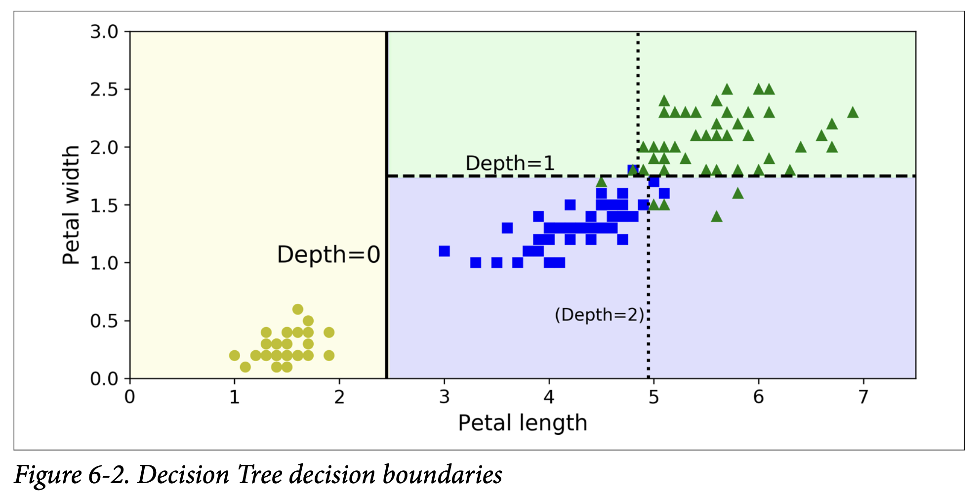
  • The root node (petal length ≤ 2.45 cm) creates the first thick vertical split. Everything to the left is classified as Setosa (pure).
  • The area to the right is impure, so the depth-1 right node splits it further with a horizontal line (petal width ≤ 1.75 cm).
  • Since max_depth=2, the tree stops there. The resulting regions are rectangular (or hyperrectangles in higher dimensions).
  • If max_depth were 3, the two depth-2 nodes could be split further, adding more boundaries (dotted lines in the figure).

• Model Interpretation: White Box vs. Black Box (Sidebar, page 178):

  • Decision Trees are very intuitive and their decisions are easy to interpret. They are often called white box models. You can see the rules.
  • In contrast, Random Forests or Neural Networks are often considered black box models. They can make great predictions, but it’s harder to explain in simple terms why a specific prediction was made.
  • Decision Trees provide simple classification rules that can even be applied manually.

(Page 178-179: Estimating Class Probabilities)

Decision Trees can also estimate the probability that an instance belongs to a particular class k.

• How it works:
  1. Traverse the tree to find the leaf node for the instance.
  2. Return the ratio of training instances of class k in that leaf node.
• Example (page 179): Flower with petal length 5 cm, petal width 1.5 cm.
  1. Petal length > 2.45 cm (False for root) -> go to depth-1 right node.
  2. Petal width ≤ 1.75 cm (True for this node) -> go to depth-2 left node (the one that predicts Versicolor).
  3. This leaf node has value = [0, 49, 5], meaning 0 Setosa, 49 Versicolor, 5 Virginica, out of 54 samples.
  • Probabilities:
    • P(Setosa) = 0/54 = 0%
    • P(Versicolor) = 49/54 ≈ 90.7%
    • P(Virginica) = 5/54 ≈ 9.3%
• Scikit-Learn code: tree_clf.predict_proba([[5, 1.5]]) gives array([[0. , 0.90740741, 0.09259259]]) tree_clf.predict([[5, 1.5]]) gives array([1]) (class 1 is Versicolor).
• Important Note: The estimated probabilities are the same for any point that falls into the same leaf node’s region (e.g., the bottom-middle rectangle in Figure 6-2). This can sometimes be a limitation if fine-grained probability estimates are needed. Even if a flower had petal length 6cm and width 1.5cm (making it seem more likely Virginica by intuition, if it were near the boundary with Virginica region), it would still get the same probabilities if it landed in that same leaf node.

(Page 179: The CART Training Algorithm)

Scikit-Learn uses the Classification and Regression Tree (CART) algorithm to train (or “grow”) Decision Trees.

• How it works (Greedy Approach):

  1. It first splits the training set into two subsets using a single feature k and a threshold tₖ (e.g., “petal length ≤ 2.45 cm”).
  2. How does it choose k and tₖ? It searches for the pair (k, tₖ) that produces the purest subsets, weighted by their size.
     • Purity is measured by Gini impurity (or entropy, which we’ll see).
     • Equation 6-2: CART cost function for classification J(k, tₖ) = (m_left / m) * G_left + (m_right / m) * G_right
       • m_left, m_right: Number of instances in the left/right subset after the split.
       • m: Total number of instances.
       • G_left, G_right: Gini impurity of the left/right subset.
       • What this cost function is ultimately trying to achieve: Find the feature and threshold that minimize this weighted average impurity of the child nodes. It wants the “cleanest” possible split.
  3. Recursion: Once the algorithm splits the set in two, it splits the subsets using the same logic, then the sub-subsets, and so on, recursively.

• Stopping Conditions (When to stop splitting/recursing):

  • Reaches max_depth (hyperparameter).
  • Cannot find a split that will reduce impurity further.
  • Other hyperparameters controlling stopping:
    • min_samples_split: Minimum number of samples a node must have before it can be split.
    • min_samples_leaf: Minimum number of samples a leaf node must have.
    • min_weight_fraction_leaf: Same as min_samples_leaf but as a fraction of total weighted instances.
    • max_leaf_nodes: Maximum number of leaf nodes. These are all regularization hyperparameters.

• Greedy Nature (Scorpion Icon, page 180):

  • CART is a greedy algorithm. At each step, it searches for the locally optimal split at the current level. It doesn’t look ahead to see if a less optimal split now might lead to an even better overall tree (lower total impurity) a few levels down.
  • A greedy algorithm often produces a solution that’s reasonably good, but not guaranteed to be globally optimal.
  • Finding the truly optimal tree is an NP-Complete problem (computationally very hard, requires O(exp(m)) time), so we settle for a “reasonably good” greedy solution.

(Page 180-181: Computational Complexity & Gini vs. Entropy)

• Prediction Complexity:

  • Traversing a Decision Tree from root to leaf takes roughly O(log₂(m)) nodes for a balanced tree (where m is number of instances).
  • Each node checks one feature.
  • So, overall prediction complexity is O(log₂(m)), independent of the number of features n. Predictions are very fast!

• Training Complexity:

  • At each node, CART compares all features (or max_features) on all samples in that node. This results in a training complexity of roughly O(n × m log₂(m)).
  • For small training sets (< few thousand), Scikit-Learn can speed up training by presorting data (presort=True parameter, though this is deprecated and will be removed; Scikit-learn now often sorts internally when beneficial). For larger sets, presorting slows it down.

• Gini Impurity or Entropy? (Page 180):

  • By default, CART uses Gini impurity. You can set criterion="entropy" to use entropy as the impurity measure instead.
  • Entropy (Equation 6-3, page 181): Hᵢ = - Σₖ (pᵢ,ₖ * log₂(pᵢ,ₖ)) (sum over classes k where pᵢ,ₖ ≠ 0)
    • Originated in thermodynamics (molecular disorder). In information theory (Shannon), it measures average information content.
    • Entropy is 0 if a set contains instances of only one class (pure).
    • What it’s ultimately trying to achieve: Similar to Gini, it measures the “mixed-up-ness” or uncertainty in a node. Lower entropy means less uncertainty/more purity.
  • Gini vs. Entropy: Does it matter?
    • Mostly, no. They lead to similar trees.
    • Gini is slightly faster to compute, so it’s a good default.
    • When they differ: Gini tends to isolate the most frequent class in its own branch of the tree. Entropy tends to produce slightly more balanced trees.

(Page 181-182: Regularization Hyperparameters)

Decision Trees make very few assumptions about the data (they are nonparametric models – the number of parameters isn’t fixed before training, the model structure adapts to the data).

• If left unconstrained, they will fit the training data very closely, likely overfitting.
• To avoid this, we need to regularize by restricting their freedom during training.
• Key Regularization Hyperparameters in DecisionTreeClassifier:
  • max_depth: Maximum depth of the tree. (Default is None = unlimited). Reducing this is a common way to regularize.
  • min_samples_split: Minimum samples a node needs to be split.
  • min_samples_leaf: Minimum samples a leaf node must have.
  • min_weight_fraction_leaf: As min_samples_leaf, but as a fraction.
  • max_leaf_nodes: Limits the total number of leaf nodes.
  • max_features: Max number of features evaluated for splitting at each node.
  • Increasing min_* hyperparameters or reducing max_* hyperparameters will regularize the model.
• Figure 6-3 (page 182): Shows the effect on the moons dataset.

  

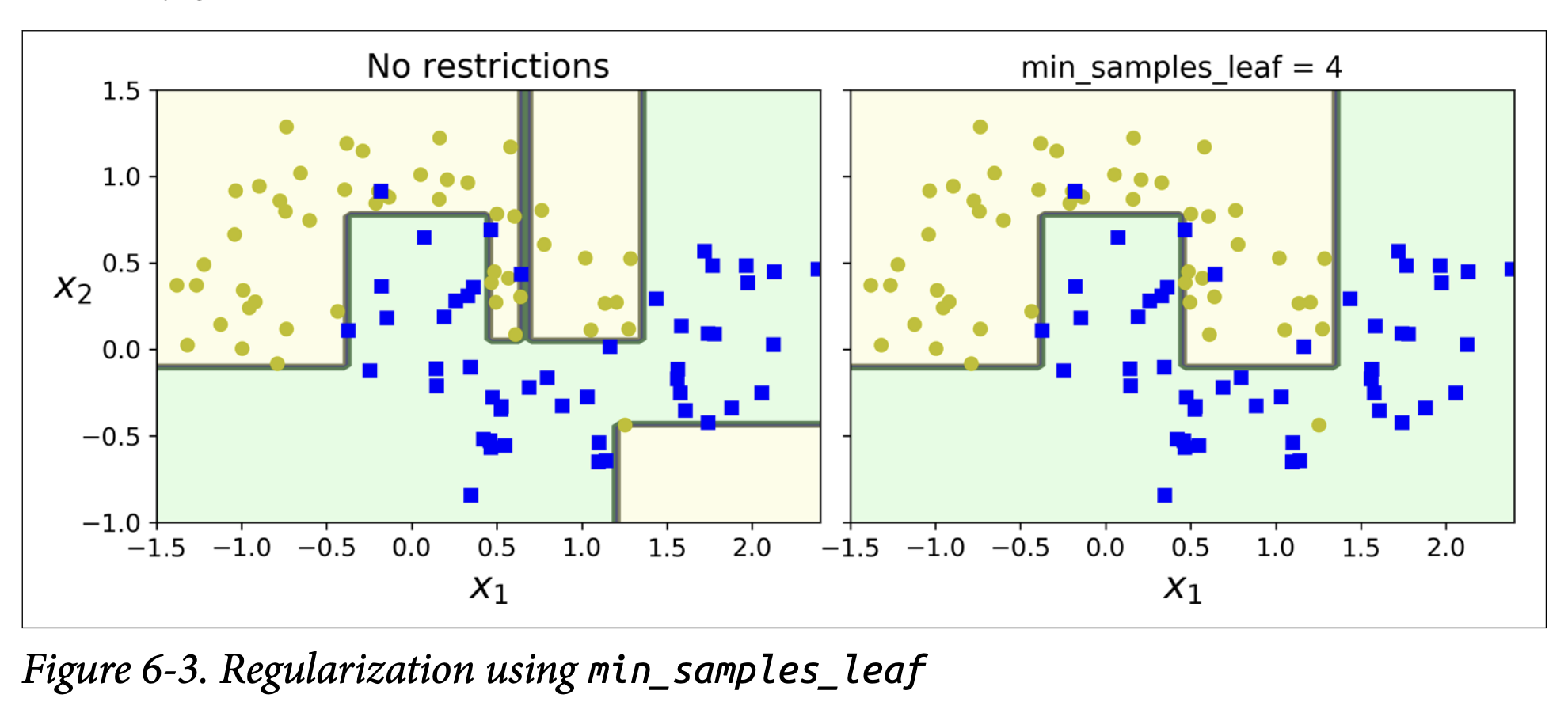
  • Left: Default hyperparameters (no restrictions) -> Overfitting (wiggly boundary).
  • Right: min_samples_leaf=4 -> Simpler, smoother boundary, likely generalizes better.
• Pruning (Scorpion Icon, page 182):
  • Some algorithms work by first training the tree without restrictions, then pruning (deleting) unnecessary nodes.
  • A node is considered unnecessary if the purity improvement it provides is not statistically significant (e.g., using a chi-squared test to check if improvement is just by chance). If p-value > threshold, prune.

(Page 183-184: Regression with Decision Trees)

Decision Trees can also do regression using DecisionTreeRegressor.

• Example: Training on a noisy quadratic dataset with max_depth=2.
• Figure 6-4 (A Decision Tree for regression): Looks similar to a classification tree.

  

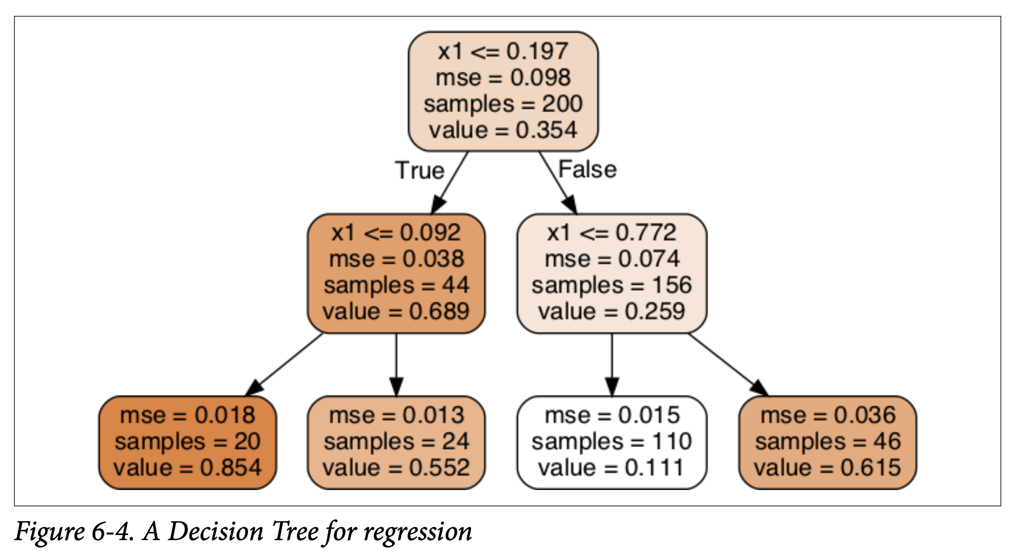
  • Main difference: Instead of predicting a class in each node, it predicts a value.
  • The value predicted at a leaf node is the average target value of the training instances that fall into that leaf.
  • The mse attribute in each node shows the mean squared error of the training instances in that node, relative to the average value of that node.
• Predictions (Figure 6-5, page 184):
  • The predictions are piecewise constant. For any region defined by a leaf node, the prediction is the average value of the training instances in that region.
  • Increasing max_depth leads to more steps in the prediction function, fitting the training data more closely.
• CART Algorithm for Regression (Equation 6-4, page 184):
  • Works mostly the same way as for classification.
  • Difference: Instead of minimizing impurity (Gini/entropy), it tries to split the training set in a way that minimizes the MSE.
  • J(k, tₖ) = (m_left / m) * MSE_left + (m_right / m) * MSE_right
  • It wants to make the instances within each resulting region as close as possible to the mean value of that region.
• Regularization (Figure 6-6, page 184):
  • Just like classification trees, regression trees are prone to overfitting if unregularized (left plot).
  • Setting min_samples_leaf=10 (right plot) gives a much more reasonable, smoother model.

(Page 185-186: Instability of Decision Trees)

Decision Trees have many great qualities (simple, interpretable, versatile, powerful). But they have limitations.

1. Sensitivity to Training Set Rotation (Orthogonal Boundaries - Figure 6-7, page 185):

   

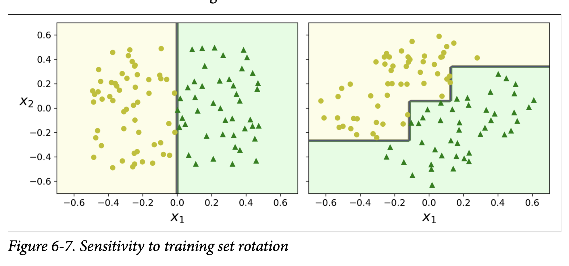
   • Decision Trees prefer to create orthogonal decision boundaries (splits are perpendicular to an axis).
   • If your dataset is rotated, a simple linear boundary in the rotated space might require a complex, step-like boundary for the Decision Tree.
   • The left plot shows a tree easily splitting unrotated data. The right shows a convoluted boundary for data rotated 45°.
   • The model on the right might not generalize well.
   • One way to limit this: Use Principal Component Analysis (PCA, Chapter 8) to orient data better first.

2. Sensitivity to Small Variations in Training Data (Figure 6-8, page 186):

   • This is a major issue. Decision Trees are very sensitive to small changes in the training data.
   • Example: Remove one instance (the widest Iris versicolor) from the Iris dataset and retrain. The resulting tree (Figure 6-8) can look very different from the original (Figure 6-2).
   • Since the CART algorithm used by Scikit-Learn is stochastic (randomly selects features to evaluate at nodes if max_features is less than total features, or how ties are broken), you might get different models even on the same training data unless you set random_state.

How to limit this instability? Random Forests (Chapter 7!) average predictions over many trees, which greatly helps reduce this variance and instability.

And that’s the essence of Decision Trees! They work by recursively partitioning the data based on simple questions about features, aiming to create purer (for classification) or more homogeneous (for regression) subsets. They are interpretable but can be unstable and prone to overfitting if not regularized.

Any thoughts or questions on how these trees make decisions or how they are built? The idea of recursive partitioning and measuring purity/error at each step is central.

Glossary

Q. Is backtracking used while training decision trees using CART algorithm in machine learning?

Yes, absolutely! The process of building a decision tree, especially using algorithms like CART (Classification and Regression Trees), shares a very strong conceptual similarity with recursive backtracking, particularly the divide-and-conquer aspect and the exploration of choices.

Here’s how they relate:

1. Recursive Partitioning (Divide and Conquer):

   • Decision Trees: At each node, the algorithm searches for the “best” feature and the “best” split point for that feature to divide the current dataset into two or more subsets. This partitioning is done recursively.
   • Backtracking/Recursion: We break a problem down into smaller sub problems.

2. Making a Sequence of Decisions:

   • Decision Trees: Building a tree is a sequence of decisions:
     • Which feature to split on at the current node?
     • What value of that feature to use as the split point?
   • Backtracking: We make a sequence of choices to build a potential solution.

3. Exploring Choices (Greedy vs. Exhaustive):

   • CART (Typically Greedy): At each node, CART makes a locally optimal decision. It searches for the single feature and split point that currently gives the best improvement in purity (e.g., Gini impurity, entropy for classification; variance reduction for regression). It commits to this split and then recursively processes the resulting child nodes. It doesn’t typically “backtrack” in the sense of undoing a split if it later turns out to be globally suboptimal. This greedy nature is why decision trees can sometimes find solutions that aren’t the absolute global optimum but are good and fast to compute.
   • Pure Backtracking (Exhaustive): Would explore all possible sequences of splits to find the globally best tree. This is computationally infeasible for most datasets.

4. Stopping Conditions (Base Cases):

   • Decision Trees: Recursion stops when:
     • A node is “pure” (all samples belong to one class).
     • A pre-defined maximum depth is reached.
     • The number of samples in a node is below a threshold.
     • No split further improves purity.
   • Backtracking: Recursion stops when:
     • A complete solution is found.
     • A dead end is reached (no valid next choice).

5. Pruning (Analogous to Constraint Checking/Pruning in Backtracking):

   • Decision Trees: After a large tree is grown (often greedily), a “pruning” step is often applied. This is where the tree might be “simplified” by removing branches that don’t contribute much to overall accuracy or that lead to overfitting. This is somewhat like backtracking deciding a path is not fruitful, but it’s typically done after the initial greedy construction.
   • Backtracking: We “prune” branches of the search space if a partial solution violates constraints.

Where they differ significantly:

• Goal:

  • Backtracking (as we discussed): Often aims to find all solutions or one solution that satisfies constraints (e.g., N-Queens, Sudoku).
  • Decision Tree (CART): Aims to build a model that generalizes well to unseen data by finding optimal decision boundaries.

• Nature of “Undo”:

  • Backtracking: The “undo” is fundamental to explore different branches of the same problem instance to find different discrete solutions.
  • CART: Typically doesn’t “undo” a split choice in its main growing phase. The “undo” equivalent is more like the post-hoc pruning process, where parts of the already-built tree are removed.

So, in summary:

The recursive, divide-and-conquer nature of building a decision tree by repeatedly finding the best split is very similar to the recursive calls in backtracking. Both explore a “tree” of possibilities.

However, CART’s typical implementation is greedy in its choice of splits at each node, whereas the backtracking problems we’ve discussed (like N-Queens for all solutions) are more exhaustive in exploring valid choices. If CART were to try and find the globally optimal decision tree by trying every possible sequence of splits and then backtracking, it would be computationally intractable.

So, while the recursive structure is similar, the search strategy (greedy vs. exhaustive with backtracking) and the ultimate goal are different. The core idea of recursively breaking down the problem based on choices is a shared theme.