The Big Picture Goal:

We want our machine learning models to make good predictions. To do this, we define a loss function (or cost function) that measures how “bad” our model’s predictions are compared to the true values.

• Training = Minimizing Loss: Training a model means finding the model parameters (like weights w and biases b) that make this loss function as small as possible.
• Calculus as a Tool for Minimization: Derivatives (and their extensions like gradients) tell us the rate of change or the slope of a function.
  • If we know the slope of our loss function with respect to our model parameters, we know which “direction” to tweak those parameters to decrease the loss. This is the essence of Gradient Descent.

So, all this calculus is ultimately about finding an efficient way to “walk downhill” on our loss function surface to find the parameter values that give the lowest error.

Now, let’s look at the paper.

(Section 1 - Introduction)

• The paper acknowledges that derivatives are critical for ML, especially deep neural networks, which are trained by optimizing a loss function.

• It mentions that while modern libraries have “automatic differentiation,” understanding the underlying matrix calculus helps to “grok academic papers” and understand what’s happening “under the hood.”

• It gives an example of a single neuron’s activation:

  • z(x) = w · x + b (affine function: dot product of weights w with input x, plus a bias b).
  • Followed by an activation function, e.g., max(0, z(x)) (ReLU).

• Key statement on training: “Training this neuron means choosing weights w and bias b so that we get the desired output for all N inputs x. To do that, we minimize a loss function… All of those [gradient descent methods] require the partial derivative (the gradient) of activation(x) with respect to the model parameters w and b. Our goal is to gradually tweak w and b so that the overall loss function keeps getting smaller…”

  • What this is ultimately trying to achieve: Use the gradient (which calculus helps us find) to iteratively adjust w and b to reduce the model’s error.

• The introduction to the paper’s goal: “…rederive and rediscover some key matrix calculus rules in an effort to explain them… There aren’t dozens of new rules to learn; just a couple of key concepts.” This is encouraging!

Let’s proceed to Section 2: Review: Scalar derivative rules (Page 4 of the paper). This should be a good refresher. Are you ready to look at these basic rules? We can take it slow and make sure each one makes sense.

Alright, let’s dive into Section 2: Review: Scalar derivative rules from the Parr & Howard paper (page 4, extending to the table on page 5).

This section is a quick refresher of the basic derivative rules you likely encountered in a first calculus course. The core idea of a derivative for a function of a single variable, f(x), is to find its instantaneous rate of change or the slope of the tangent line at any given point x.

What we are ultimately trying to achieve with derivatives (in an ML context): We want to know how a small change in an input (like a model parameter θ or an input feature x) will affect the output of a function (like the loss function J(θ) or an activation function a(z)). If the derivative is large and positive, a small increase in the input leads to a large increase in the output. If it’s negative, an increase in input leads to a decrease in output. If it’s zero, the function is momentarily flat at that point (which could indicate a minimum, maximum, or a plateau).

Let’s look at the rules presented in the table on page 5:

1. Constant Rule:

   • Rule: f(x) = c (where c is a constant)
   • Scalar derivative notation: d/dx (c) = 0
   • Example: d/dx (99) = 0
   • What it’s ultimately trying to achieve: A constant function doesn’t change, no matter what x is. So, its rate of change (slope) is always zero. Think of a flat horizontal line – its slope is 0.

2. Multiplication by Constant Rule:

   • Rule: f(x) = cf(x) (actually, it should be g(x) = c * f(x))
   • Scalar derivative notation: d/dx (c * f(x)) = c * (df/dx)
   • Example: d/dx (3x) = 3 * (d/dx (x)) = 3 * 1 = 3
   • What it’s ultimately trying to achieve: If you scale a function by a constant, its rate of change (slope) at any point is also scaled by that same constant. The shape of the change is the same, just amplified or shrunk.

3. Power Rule:

   • Rule: f(x) = xⁿ
   • Scalar derivative notation: d/dx (xⁿ) = nxⁿ⁻¹
   • Example: d/dx (x³) = 3x³⁻¹ = 3x²
   • What it’s ultimately trying to achieve: This rule tells us how functions involving powers of x change. For x³, the slope isn’t constant; it changes depending on x. At x=1, slope is 3. At x=2, slope is 3*(2)² = 12.

4. Sum Rule:

   • Rule: h(x) = f(x) + g(x)
   • Scalar derivative notation: d/dx (f(x) + g(x)) = (df/dx) + (dg/dx)
   • Example: d/dx (x² + 3x) = (d/dx x²) + (d/dx 3x) = 2x + 3
   • What it’s ultimately trying to achieve: The rate of change of a sum of functions is the sum of their individual rates of change. If one part is changing quickly and another slowly, the sum changes according to the combined effect.

5. Difference Rule:

   • Rule: h(x) = f(x) - g(x)
   • Scalar derivative notation: d/dx (f(x) - g(x)) = (df/dx) - (dg/dx)
   • Example: d/dx (x² - 3x) = (d/dx x²) - (d/dx 3x) = 2x - 3
   • What it’s ultimately trying to achieve: Similar to the sum rule, the rate of change of a difference is the difference of the rates of change.

6. Product Rule:

   • Rule: h(x) = f(x)g(x)
   • Scalar derivative notation: d/dx (f(x)g(x)) = f(x)(dg/dx) + (df/dx)g(x)
   • Example: d/dx (x² * x) (where f(x)=x², g(x)=x)
     • = x² * (d/dx x) + (d/dx x²) * x
     • = x² * 1 + 2x * x = x² + 2x² = 3x²
     • (This is consistent with d/dx (x³) = 3x²)
   • What it’s ultimately trying to achieve: When two functions are multiplied, a change in x affects both. The overall rate of change depends on how g(x) changes (weighted by f(x)) plus how f(x) changes (weighted by g(x)).

7. Chain Rule (for single variable nested functions):

   • Rule: h(x) = f(g(x)) (a function f applied to the output of another function g)
   • Scalar derivative notation: d/dx f(g(x)) = (df/du) * (du/dx), where u = g(x).
     • The paper writes this as df(u)/du * du/dx.
   • Example: d/dx ln(x²)
     • Let u = g(x) = x². Then f(u) = ln(u).
     • du/dx = d/dx (x²) = 2x.
     • df/du = d/du (ln(u)) = 1/u.
     • So, d/dx ln(x²) = (1/u) * (2x) = (1/x²) * (2x) = 2x/x² = 2/x.
   • What it’s ultimately trying to achieve: It tells us how to find the rate of change of a composite function. How much does the outer function f change with respect to its input u (df/du), multiplied by how much that inner input u changes with respect to the original variable x (du/dx). It “chains” the rates of change together. This rule is extremely important for neural networks because they are essentially deeply nested functions, and backpropagation is an application of the chain rule.

The paper also mentions (bottom of page 4, top of page 5):

• The notation d/dx can be thought of as an operator that takes a function f(x) and gives you its derivative df/dx.
• This operator view is helpful because the operator is distributive (d/dx (f+g) = df/dx + dg/dx) and lets you pull out constants (d/dx (cf) = c * df/dx). This simplifies taking derivatives of complex expressions, like their example: d/dx (9(x + x²)) = 9 * d/dx (x + x²) = 9 * (d/dx x + d/dx x²) = 9 * (1 + 2x) = 9 + 18x.

This review of scalar derivative rules is foundational. For deep learning and training models with Gradient Descent, we are constantly asking: “If I wiggle this weight/bias a tiny bit, how much does my loss function change?” Derivatives give us the answer to that question.

Section 3: Introduction to vector calculus and partial derivatives

This section transitions us from functions of a single variable (f(x)) to functions of multiple variables (e.g., f(x, y)). Neural network layers often have many inputs (features) and many parameters (weights, biases), so we need to be able to talk about how the output changes when we wiggle one specific input or parameter, while keeping others constant.

• Functions of Multiple Parameters:

  • Instead of f(x), we now consider f(x, y). For example, the product xy.
  • If we want to know its derivative, the question is “derivative with respect to what?” With respect to x, or with respect to y? The change in xy will be different depending on which variable we “wiggle.”

• Partial Derivatives:

  • When we have a function of multiple variables, we compute partial derivatives.
  • The notation changes from d/dx to ∂/∂x (using a stylized ’d’, often called “del” or “curly d”).
  • ∂f(x,y)/∂x: This is the partial derivative of f(x,y) with respect to x.
    • What it’s ultimately trying to achieve: It tells us the rate of change of the function f if we change x by a tiny amount, while holding all other variables (in this case, y) constant. You treat y as if it were just a number.
  • ∂f(x,y)/∂y: This is the partial derivative of f(x,y) with respect to y.
    • What it’s ultimately trying to achieve: It tells us the rate of change of f if we change y by a tiny amount, while holding x constant.

• Example from the paper: f(x, y) = 3x²y

  • Partial derivative with respect to x (∂f/∂x):
    • Treat y (and 3) as constants.
    • ∂/∂x (3x²y) = 3y * (∂/∂x x²) = 3y * (2x) = 6yx.
    • Intuition: If y is fixed, say y=2, then f(x,2) = 6x². The derivative d/dx (6x²) = 12x. Our partial derivative 6yx gives 6(2)x = 12x. It matches!
  • Partial derivative with respect to y (∂f/∂y):
    • Treat x (and 3x²) as constants.
    • ∂/∂y (3x²y) = 3x² * (∂/∂y y) = 3x² * 1 = 3x².
    • Intuition: If x is fixed, say x=1, then f(1,y) = 3y. The derivative d/dy (3y) = 3. Our partial derivative 3x² gives 3(1)² = 3. It matches!

• The Gradient (∇f):

  • For a function of multiple variables, like f(x,y), we can organize all its partial derivatives into a vector. This vector is called the gradient of f, denoted by ∇f (nabla f).
  • For f(x,y) = 3x²y, the paper writes: ∇f(x, y) = [∂f/∂x, ∂f/∂y] = [6yx, 3x²]
  • What the gradient is ultimately trying to achieve: The gradient vector ∇f at a specific point (x₀, y₀) points in the direction of the steepest ascent (fastest increase) of the function f at that point. Its magnitude ||∇f|| tells you the rate of increase in that direction.
  • In machine learning, our loss function J(θ) depends on many parameters θ₁, θ₂, ..., θₙ. The gradient ∇J(θ) will be a vector [∂J/∂θ₁, ∂J/∂θ₂, ..., ∂J/∂θₙ].
  • Gradient Descent uses this: it calculates ∇J(θ) and then takes a step in the opposite direction (-∇J(θ)) to go “downhill” and reduce the loss.

This section essentially extends the concept of a derivative (rate of change/slope) from single-variable functions to multi-variable functions by considering the rate of change with respect to each variable individually, holding others constant. The gradient then bundles all these partial rates of change into a single vector that gives us the “overall” direction of steepest increase.

Section 4: Matrix calculus

This is where things get a bit more generalized. So far:

• Scalar derivative: df/dx (function of one variable, derivative is a scalar).
• Vector calculus (gradient): ∇f(x,y) = [∂f/∂x, ∂f/∂y] (function of multiple scalar variables x, y, output is a scalar f, gradient is a vector of partials).

Matrix calculus deals with derivatives when:

1. The input is a vector (e.g., x = [x₁, x₂]).
2. The output can also be a vector (e.g., y = [f₁(x), f₂(x)]).

• From One Function to Many Functions:
  • The paper keeps f(x, y) = 3x²y from the previous section.
  • It introduces another function g(x, y) = 2x + y⁸.
  • We can find the gradient of g just like we did for f:
    • ∂g/∂x = ∂/∂x (2x + y⁸) = 2 (treating y⁸ as constant)
    • ∂g/∂y = ∂/∂y (2x + y⁸) = 8y⁷ (treating 2x as constant)
    • So, ∇g(x, y) = [2, 8y⁷].

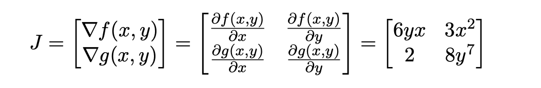
• The Jacobian Matrix (J):

  • When we have multiple functions (say, f and g), each of which can depend on multiple input variables (say, x and y), we can organize their gradients into a matrix. This matrix is called the Jacobian matrix (or just the Jacobian).

  • If we have two functions f(x,y) and g(x,y), the Jacobian J (using the paper’s “numerator layout” where gradients are rows) is formed by stacking their gradient vectors: J = [ ∇f(x, y) ] = [ ∂f/∂x ∂f/∂y ] [ ∇g(x, y) ] [ ∂g/∂x ∂g/∂y ]

    So for f(x,y) = 3x²y and g(x,y) = 2x + y⁸, the Jacobian is: J = [ 6yx 3x² ] [ 2 8y⁷ ]

  • What the Jacobian is ultimately trying to achieve: It captures all the first-order partial derivatives of a vector-valued function (a function that outputs a vector of values) with respect to a vector of input variables.

    • Each row i tells you how function fᵢ changes with respect to each input variable.
    • Each column j tells you how all output functions change with respect to input variable xⱼ.
    • Essentially, if you have m functions and n input variables, the Jacobian is an m x n matrix where the entry Jᵢⱼ = ∂fᵢ/∂xⱼ.

• Layouts (Numerator vs. Denominator):

  • The paper notes: “there are multiple ways to represent the Jacobian.” They use “numerator layout” (where ∇f is a row vector, and the Jacobian stacks these row vectors).
  • Other sources might use “denominator layout,” which is essentially the transpose of the numerator layout Jacobian. It’s important to be aware of this when consulting different texts, as the shapes of matrices in equations will change accordingly. The paper sticks to numerator layout. Example given (page 7, top): Transpose of our Jacobian above is [ 6yx 2 ] [ 3x² 8y⁷ ]

This Jacobian matrix is a fundamental tool when dealing with transformations between vector spaces in calculus, and it plays a key role in the chain rule for vector functions, which is vital for backpropagation in neural networks with multiple layers and multiple neurons per layer.

The main idea here is organization:

• Gradient: Organizes partial derivatives of a single scalar-output function with respect to its multiple inputs into a vector.
• Jacobian: Organizes gradients of multiple scalar-output functions (or equivalently, partial derivatives of a single vector-output function) into a matrix.

Great! Understanding the Jacobian as an organized collection of partial derivatives is a key step.

Section 4.1: Generalization of the Jacobian (page 7 of the Parr & Howard paper).

This section formalizes the Jacobian for a general case where you have a vector of functions, y = f(x), where x is an input vector and y is an output vector.

• Vector Notation:

  • Input vector x has n elements: x = [x₁, x₂, ..., xₙ]ᵀ (they assume column vectors by default).
  • Output vector y has m scalar-valued functions: y = [f₁(x), f₂(x), ..., fₘ(x)]ᵀ. Each fᵢ(x) takes the whole vector x as input and returns a scalar.

• The Jacobian Matrix ∂y/∂x: The paper defines the Jacobian as a stack of m gradients (one for each output function fᵢ). Since they use numerator layout (where each gradient ∇fᵢ(x) is a row vector of partials with respect to the components of x), the Jacobian becomes an m x n matrix:

  ∂y/∂x = [ ∇f₁(x) ] = [ ∂f₁/∂x₁ ∂f₁/∂x₂ ... ∂f₁/∂xₙ ] [ ∇f₂(x) ] [ ∂f₂/∂x₁ ∂f₂/∂x₂ ... ∂f₂/∂xₙ ] [ ... ] [ ... ... ... ... ] [ ∇fₘ(x) ] [ ∂fₘ/∂x₁ ∂fₘ/∂x₂ ... ∂fₘ/∂xₙ ]

  • Rows: Each row i of the Jacobian corresponds to one output function fᵢ(x) and contains all the partial derivatives of that specific output function with respect to each of the input variables x₁, x₂, ..., xₙ. So, row i is ∇fᵢ(x).
  • Columns: Each column j of the Jacobian corresponds to one input variable xⱼ and contains all the partial derivatives of each of the output functions f₁, f₂, ..., fₘ with respect to that specific input variable xⱼ.

  What the Jacobian ∂y/∂x is ultimately trying to achieve: It describes how each component of the output vector y changes in response to a small change in each component of the input vector x. It’s a complete map of all the first-order sensitivities between the inputs and outputs.

• Visualizing Jacobian Shapes (diagram on page 8): This is a handy diagram to remember the dimensions based on the nature of input x and output f (or y):

  • Scalar input x, Scalar output f: Derivative ∂f/∂x is a scalar. (This is standard Calc 1).
  • Vector input x, Scalar output f: Derivative ∂f/∂x (which is ∇f) is a row vector (1 x n) in numerator layout.
  • Scalar input x, Vector output f: Derivative ∂f/∂x is a column vector (m x 1). (Each ∂fᵢ/∂x is a scalar, stacked up).
  • Vector input x, Vector output f: Derivative ∂f/∂x (the Jacobian) is an m x n matrix.

• Example: Jacobian of the Identity Function (page 8):

  • If y = f(x) = x, then each output component yᵢ is just equal to the corresponding input component xᵢ (so fᵢ(x) = xᵢ). Here, m=n.
  • Let’s find ∂fᵢ/∂xⱼ = ∂xᵢ/∂xⱼ:
    • If i = j, then ∂xᵢ/∂xᵢ = 1 (the derivative of x₁ with respect to x₁ is 1).
    • If i ≠ j, then ∂xᵢ/∂xⱼ = 0 (e.g., x₁ does not change when x₂ changes, because they are independent input components, so ∂x₁/∂x₂ = 0).
  • When you assemble these into the Jacobian matrix, you get 1s on the main diagonal and 0s everywhere else. This is the Identity Matrix (I).
  • ∂x/∂x = I
  • What this ultimately means: If you wiggle an input xⱼ by a small amount, only the corresponding output yⱼ wiggles by that same amount, and other outputs yᵢ (where i≠j) don’t change at all. This makes perfect sense for the identity function.

This section firmly establishes the Jacobian matrix as the way to represent the derivative of a vector function with respect to a vector input. It’s the matrix that holds all the individual “slopes” that connect changes in each input dimension to changes in each output dimension.

This general form of the Jacobian will be crucial when we get to the vector chain rule later, which is how backpropagation efficiently calculates gradients through multiple layers of a neural network, where each layer can be seen as a vector function taking a vector input.

Section 4.2: Derivatives of vector element-wise binary operators (Pages 9-11).

The Big Picture of This Section:

Neural networks involve many operations on vectors: adding an input vector to a bias vector, multiplying activations by weights, etc. Often, these operations are element-wise – meaning the operation is applied independently to corresponding elements of the input vectors to produce an element of the output vector.

• Example: If w = [w₁, w₂] and x = [x₁, x₂], then w + x = [w₁ + x₁, w₂ + x₂]. The first element of the output only depends on the first elements of the inputs, and so on.

This section aims to figure out:

• If we have an output vector y that’s a result of an element-wise operation between two input vectors w and x (e.g., y = w + x or y = w * x), how does y change if we wiggle w? (This gives us the Jacobian ∂y/∂w).
• And how does y change if we wiggle x? (This gives us the Jacobian ∂y/∂x).

What we are ultimately trying to achieve here is to find simplified forms for these Jacobians, because for element-wise operations, many of the terms in the full Jacobian matrix will turn out to be zero.

Breaking it Down (Page 9):

The paper starts with the general form: y = f(w) ⊙ g(x).

• w and x are input vectors.
• f(w) and g(x) are functions that produce vectors of the same size.
• ⊙ represents any element-wise binary operator (like +, -, element-wise *, element-wise /).
• y is the output vector. So, yᵢ = fᵢ(w) ⊙ gᵢ(x). The i-th element of y depends only on the i-th element processing of w and x.

The full Jacobian ∂y/∂w would be a matrix where element (i,j) is ∂yᵢ/∂wⱼ (how the i-th output element yᵢ changes with respect to the j-th input element wⱼ from vector w). Similarly for ∂y/∂x.

The “Furball” and the Simplification (Page 10):

The general Jacobian matrix for such an operation (shown at the bottom of page 9) looks complicated – a “furball,” as the paper says.

However, because the operations are element-wise, there’s a huge simplification:

• yᵢ (the i-th element of the output) only depends on wᵢ (the i-th element of w) and xᵢ (the i-th element of x).
• yᵢ does not depend on wⱼ if j ≠ i.
• yᵢ does not depend on xⱼ if j ≠ i.

What does this mean for the Jacobian ∂y/∂w? Consider ∂yᵢ/∂wⱼ:

• If j ≠ i (we are looking at an off-diagonal element of the Jacobian): Since yᵢ does not depend on wⱼ, its derivative ∂yᵢ/∂wⱼ must be zero.
• If j = i (we are looking at a diagonal element of the Jacobian): Then ∂yᵢ/∂wᵢ will generally be non-zero, and it’s just the derivative of the i-th scalar operation fᵢ(wᵢ) ⊙ gᵢ(xᵢ) with respect to wᵢ (treating xᵢ as a constant for this partial derivative).

The Result: Diagonal Jacobians! This means that for element-wise operations, the Jacobian matrices ∂y/∂w and ∂y/∂x are diagonal matrices. A diagonal matrix has non-zero values only along its main diagonal, and zeros everywhere else.

The paper introduces the “element-wise diagonal condition”: fᵢ(w) should only access wᵢ and gᵢ(x) should only access xᵢ. This is precisely what happens in simple element-wise vector operations.

So, the Jacobian ∂y/∂w simplifies to (middle of page 10): ∂y/∂w = diag( ∂/∂w₁ (f₁(w₁) ⊙ g₁(x₁)), ∂/∂w₂ (f₂(w₂) ⊙ g₂(x₂)), ..., ∂/∂wₙ (fₙ(wₙ) ⊙ gₙ(xₙ)) ) Each term on the diagonal is just a scalar derivative of the i-th component operation.

What this simplification is ultimately trying to achieve: It makes calculating these Jacobians much easier. Instead of a full matrix of derivatives, we only need to calculate n scalar derivatives for the diagonal.

Special Case: f(w) = w (Page 10-11)

Very often in neural networks, one of the functions in the element-wise operation is just the identity. For example, vector addition y = w + x. Here f(w) = w (so fᵢ(wᵢ) = wᵢ) and g(x) = x (so gᵢ(xᵢ) = xᵢ).

Let’s look at y = w + x, so yᵢ = wᵢ + xᵢ.

• ∂y/∂w:
  • The i-th diagonal element is ∂/∂wᵢ (wᵢ + xᵢ). Treating xᵢ as a constant, this derivative is 1.
  • So, ∂(w+x)/∂w = diag(1, 1, ..., 1) = I (the identity matrix).
• ∂y/∂x:
  • The i-th diagonal element is ∂/∂xᵢ (wᵢ + xᵢ). Treating wᵢ as a constant, this derivative is 1.
  • So, ∂(w+x)/∂x = diag(1, 1, ..., 1) = I (the identity matrix).

The paper then lists Jacobians for common element-wise binary operations where f(w) = w (so fᵢ(wᵢ) = wᵢ):

• Addition: y = w + x

  • ∂y/∂w = I
  • ∂y/∂x = I
  • Intuition: If you wiggle w₁ by a small amount Δ, y₁ changes by Δ, and no other yⱼ changes. Same for x.

• Subtraction: y = w - x

  • ∂y/∂w = I
  • ∂y/∂x = -I (because ∂/∂xᵢ (wᵢ - xᵢ) = -1)
  • Intuition: If you wiggle x₁ by Δ, y₁ changes by -Δ.

• Element-wise Multiplication (Hadamard Product): y = w ⊗ x (so yᵢ = wᵢ * xᵢ)

  • ∂y/∂w: i-th diagonal element is ∂/∂wᵢ (wᵢ * xᵢ) = xᵢ. So, ∂y/∂w = diag(x).
  • ∂y/∂x: i-th diagonal element is ∂/∂xᵢ (wᵢ * xᵢ) = wᵢ. So, ∂y/∂x = diag(w).
  • Intuition for ∂y/∂w: If you wiggle w₁ by Δ, y₁ changes by x₁ * Δ. The change in y₁ depends on the value of x₁.

• Element-wise Division: y = w / x (so yᵢ = wᵢ / xᵢ)

  • ∂y/∂w: i-th diagonal element is ∂/∂wᵢ (wᵢ / xᵢ) = 1/xᵢ. So, ∂y/∂w = diag(1/x₁, 1/x₂, ...).
  • ∂y/∂x: i-th diagonal element is ∂/∂xᵢ (wᵢ / xᵢ) = -wᵢ / xᵢ². So, ∂y/∂x = diag(-w₁/x₁², ...).

Key Takeaway from Section 4.2: When dealing with element-wise operations between two vectors w and x to produce y, the Jacobians ∂y/∂w and ∂y/∂x are diagonal matrices. This is a huge simplification. The values on the diagonal are found by simply taking the scalar derivative of the i-th component operation with respect to the i-th component of the input vector. This section provides the rules for common operations like addition, subtraction, and element-wise multiplication/division.

This means that when we’re backpropagating gradients through such an element-wise layer, the calculations become much simpler than if we had to deal with full Jacobian matrices. We’re essentially just scaling the incoming gradients by these diagonal terms.

Section 4.3: Derivatives involving scalar expansion (Pages 11-12).

The Big Picture of This Section:

In neural networks, we often perform operations between a vector and a scalar. For example:

• Adding a scalar bias b to every element of a vector z: y = z + b.
• Multiplying every element of a vector z by a scalar learning rate η: y = η * z.

This section explains how to find the derivatives for these types of operations. The trick is to realize that these operations can be viewed as implicit element-wise operations where the scalar is “expanded” or “broadcast” into a vector of the same size as the other vector.

What we are ultimately trying to achieve here is to get rules for how the output vector y changes if we wiggle the input vector x, and how y changes if we wiggle the input scalar z.

Breaking it Down (Page 11-12):

The paper uses the example y = x + z, where x is a vector and z is a scalar.

• Implicit Expansion: This is really y = f(x) + g(z) where f(x) = x and g(z) = 1z (a vector where every element is z).
• So, yᵢ = xᵢ + z. Each element yᵢ is the sum of the corresponding xᵢ and the same scalar z.

1. Derivative with respect to the vector x: ∂y/∂x

• This fits the “element-wise diagonal condition” we just discussed.
  • fᵢ(x) = xᵢ only depends on xᵢ.
  • gᵢ(z) = z (for the i-th component) only depends on the scalar z (which is considered independent of x for this partial derivative).
• The i-th diagonal element of the Jacobian ∂y/∂x is ∂/∂xᵢ (xᵢ + z).
• Since z is treated as a constant when differentiating with respect to xᵢ, ∂z/∂xᵢ = 0.
• So, ∂/∂xᵢ (xᵢ + z) = ∂xᵢ/∂xᵢ + ∂z/∂xᵢ = 1 + 0 = 1.
• Therefore, ∂y/∂x = diag(1, 1, ..., 1) = I (the identity matrix).
• Intuition: If you wiggle xᵢ by a small amount Δ, only yᵢ changes, and it changes by Δ. This is the definition of the identity matrix’s effect.
• What this is ultimately trying to achieve: It confirms that adding a scalar to a vector shifts all elements equally, so the rate of change of each output element yᵢ with respect to its corresponding input xᵢ is 1, and there’s no cross-influence.

2. Derivative with respect to the scalar z: ∂y/∂z This is different! We are differentiating a vector output y with respect to a scalar input z. Based on the table from page 8 (or just thinking about it):

• Input: scalar z
• Output: vector y
• The derivative ∂y/∂z should be a column vector (or a vertical vector as the paper terms it). Each element of this column vector will be ∂yᵢ/∂z.
• Let’s find ∂yᵢ/∂z for yᵢ = xᵢ + z.
• When differentiating with respect to z, we treat xᵢ as a constant. So, ∂xᵢ/∂z = 0.
• ∂yᵢ/∂z = ∂/∂z (xᵢ + z) = ∂xᵢ/∂z + ∂z/∂z = 0 + 1 = 1.
• Since this is true for every i (from 1 to n, the dimension of y and x), then ∂y/∂z is a column vector of all ones.
• The paper writes this as ∂/∂z (x + z) = 1 (where 1 is the vector of ones of appropriate length).
• Intuition: If you wiggle the single scalar z by Δ, every element yᵢ of the output vector changes by Δ because z is added to every xᵢ.
• What this is ultimately trying to achieve: It shows how a single scalar change propagates to all elements of the output vector when scalar addition is involved.

Now for Scalar Multiplication: y = xz (or y = zx) This is treated as element-wise multiplication: y = x ⊗ 1z. So, yᵢ = xᵢ * z.

1. Derivative with respect to the vector x: ∂y/∂x

• Again, element-wise diagonal condition holds.
• The i-th diagonal element is ∂/∂xᵢ (xᵢ * z).
• Treat z as constant: ∂/∂xᵢ (xᵢ * z) = z * ∂xᵢ/∂xᵢ = z * 1 = z.
• So, ∂y/∂x = diag(z, z, ..., z) = zI (scalar z times the identity matrix).
• The paper writes this as ∂/∂x (xz) = diag(1z) = Iz. (Here, 1z in diag(1z) means a vector of zs, which makes more sense. If diag(z) was meant for a scalar z, it would just be z itself, not a matrix. So diag(1z) is the clearer way to express zI). My interpretation: diag(1z) means a diagonal matrix with z on every diagonal element. This is z * I.
• Intuition: If you wiggle xᵢ by Δ, yᵢ changes by z * Δ. The effect is scaled by z.

2. Derivative with respect to the scalar z: ∂y/∂z

• ∂y/∂z will be a column vector. The i-th element is ∂yᵢ/∂z.
• yᵢ = xᵢ * z. Treat xᵢ as constant.
• ∂yᵢ/∂z = ∂/∂z (xᵢ * z) = xᵢ * ∂z/∂z = xᵢ * 1 = xᵢ.
• So, ∂y/∂z is a column vector whose elements are [x₁, x₂, ..., xₙ]ᵀ, which is just the vector x.
• The paper writes this as ∂/∂z (xz) = x.
• Intuition: If you wiggle the scalar z by Δ, the i-th output yᵢ changes by xᵢ * Δ. The amount yᵢ changes depends on the value of xᵢ.
• What this is ultimately trying to achieve: It shows how a single scalar change z propagates to the output vector y, with each element yᵢ being affected proportionally to the corresponding xᵢ.

Key Takeaway from Section 4.3: Operations involving a vector and a scalar (like adding a scalar to a vector, or multiplying a vector by a scalar) can be understood by “expanding” the scalar into a vector and then applying the rules for element-wise vector operations.

• When differentiating with respect to the vector input, the Jacobian is still diagonal.
• When differentiating with respect to the scalar input, the result is a vector (not a diagonal matrix), because a single change in the scalar affects all components of the output vector.

This section helps us build up the rules needed for things like Wx + b in a neural network layer, where b might be a bias vector added element-wise, or a scalar bias broadcasted. The logic applies similarly.

Section 4.4: Vector sum reduction (Pages 12-13).

The Big Picture of This Section:

In many machine learning contexts, especially when defining loss functions, we often need to reduce a vector to a single scalar value. The most common way to do this is by summing up all the elements of the vector.

• Example: The Mean Squared Error (MSE) involves summing the squared errors for each instance. If we have a vector of squared errors, we sum them up to get a total squared error, then average.

This section focuses on finding the derivative of such a sum:

• If y = sum(f(x)), where x is an input vector and f(x) produces an output vector whose elements are then summed to get the scalar y, how does this scalar y change if we wiggle the input vector x? This will give us ∂y/∂x, which will be a gradient (a row vector, according to the paper’s convention for derivative of a scalar w.r.t. a vector).

What we are ultimately trying to achieve here is a rule for how to differentiate through a summation operation. This is critical for backpropagation, as the total loss is often a sum of losses from individual components or instances.

Breaking it Down (Page 13):

Let y = sum(f(x)) = Σᵢ fᵢ(x).

• x is an input vector [x₁, x₂, ..., xₙ].
• f(x) is a vector-valued function, producing an output vector [f₁(x), f₂(x), ..., fₚ(x)]. (Note: the paper uses n as the dimension of x and also n for the number of terms in the sum, implying p=n. Let’s assume the output vector of f(x) has p elements).
• Each fᵢ(x) could potentially depend on all elements of x (not just xᵢ). This is an important distinction from the element-wise operations earlier.
• y is the scalar sum of all elements of the vector f(x).

We want to find the gradient ∂y/∂x. This will be a row vector: ∂y/∂x = [∂y/∂x₁, ∂y/∂x₂, ..., ∂y/∂xₙ]

Let’s consider one component of this gradient, ∂y/∂xⱼ (how the sum y changes with respect to one input element xⱼ): ∂y/∂xⱼ = ∂/∂xⱼ ( Σᵢ fᵢ(x) )

Because the derivative operator is distributive over a sum, we can move it inside: ∂y/∂xⱼ = Σᵢ ( ∂fᵢ(x)/∂xⱼ )

What this means: To find how the total sum y changes when xⱼ changes, we sum up how each individual term fᵢ(x) in the sum changes when xⱼ changes.

So, the gradient vector ∂y/∂x becomes: ∂y/∂x = [ Σᵢ(∂fᵢ/∂x₁), Σᵢ(∂fᵢ/∂x₂), ..., Σᵢ(∂fᵢ/∂xₙ) ]

Example 1: y = sum(x) (Simple sum of input vector elements) Here, f(x) = x, so fᵢ(x) = xᵢ.

• ∂y/∂xⱼ = Σᵢ (∂xᵢ/∂xⱼ)
  • ∂xᵢ/∂xⱼ is 1 if i=j, and 0 if i≠j.
  • So, in the sum Σᵢ (∂xᵢ/∂xⱼ), only one term is non-zero: when i=j, the term is 1.
  • Therefore, ∂y/∂xⱼ = 1 for all j.
• This means ∂y/∂x = [1, 1, ..., 1].
• The paper writes this as ∇y = 1ᵀ (a row vector of ones).
• Intuition: If you have y = x₁ + x₂ + ... + xₙ, and you wiggle x₁ by a small amount Δ, y changes by Δ. If you wiggle x₂ by Δ, y also changes by Δ, and so on. The rate of change of y with respect to any xⱼ is 1.
• What this result ultimately achieves: It gives us a very simple rule: the derivative of the sum of a vector’s elements, with respect to that vector itself, is a vector of ones (transposed to match the gradient convention).

Example 2: y = sum(xz) (Sum of a vector multiplied by a scalar) Here, x is a vector, z is a scalar. Let f(x,z) be the vector xz (meaning fᵢ(x,z) = xᵢz). Then y = sum(f(x,z)) = Σᵢ (xᵢz).

1. Derivative with respect to the vector x: ∂y/∂x

   • The j-th component of the gradient is ∂y/∂xⱼ = Σᵢ (∂(xᵢz)/∂xⱼ).
   • ∂(xᵢz)/∂xⱼ:
     • If i = j: ∂(xⱼz)/∂xⱼ = z (treating z as constant).
     • If i ≠ j: ∂(xᵢz)/∂xⱼ = 0 (because xᵢz doesn’t depend on xⱼ).
   • So, in the sum Σᵢ (∂(xᵢz)/∂xⱼ), only the term where i=j survives, and it is z.
   • Therefore, ∂y/∂xⱼ = z for all j.
   • This means ∂y/∂x = [z, z, ..., z].
   • Intuition: If y = x₁z + x₂z + ... + xₙz, and you wiggle xⱼ by Δ, then y changes by zΔ. The rate of change is z.

2. Derivative with respect to the scalar z: ∂y/∂z (This is a scalar derivative of a scalar w.r.t a scalar)

   • y = Σᵢ (xᵢz) = z * (Σᵢ xᵢ).
   • ∂y/∂z = ∂/∂z ( z * sum(x) ).
   • Since sum(x) is treated as a constant when differentiating w.r.t. z,
   • ∂y/∂z = sum(x).
   • Intuition: If y = z * (x₁ + x₂ + ... + xₙ), and you wiggle z by Δ, then y changes by (x₁ + ... + xₙ)Δ. The rate of change is sum(x).

Key Takeaway from Section 4.4: When you differentiate a scalar sum y = sum(f(x)) with respect to the input vector x, the j-th component of the resulting gradient ∂y/∂x is the sum of how each term fᵢ(x) in the original sum changes with respect to xⱼ.

• For y = sum(x), this simplifies to ∂y/∂x = 1ᵀ.
• This rule is fundamental for backpropagation because the overall loss of a network is often a sum (or average) of losses per instance, or a sum of terms in a complex loss function. When we take the derivative of this total loss with respect to weights in earlier layers, we’ll be implicitly using this idea of differentiating through a sum.

The paper uses the notation ∇y when the output y is a scalar and the differentiation is with respect to a vector, resulting in a row vector (the gradient). It uses ∂y/∂x for the more general Jacobian when y could also be a vector.

Section 4.5: The Chain Rules

The Big Picture of This Section:

Neural networks are essentially deeply nested functions. The output of one layer becomes the input to the next, which then feeds into another, and so on, until we get the final output, and then a loss function is applied. loss = L( activation_L( ... activation_2( activation_1(X, w₁, b₁), w₂, b₂) ... ), y_true )

To train the network using gradient descent, we need to calculate how the final loss changes with respect to every single weight and bias in the entire network, even those in the very first layers. This is a monumental task if done naively.

The Chain Rule is the mathematical tool that allows us to do this efficiently.

• What it’s ultimately trying to achieve: It provides a systematic way to calculate the derivative of a composite (nested) function by breaking it down into simpler derivatives of its constituent parts and then “chaining” them together (usually by multiplication).

The paper discusses three variants, from simple to more general:

1. Single-variable chain rule (scalar function of a scalar variable).
2. Single-variable total-derivative chain rule (scalar function of a scalar variable, but with intermediate multivariate functions).
3. Vector chain rule (vector function of a vector variable). This is the most general one for neural networks.

4.5.1 Single-variable chain rule (Pages 14-17)

This is the chain rule you likely learned in basic calculus.

• Scenario: You have a function nested within another, like y = f(g(x)). For example, y = sin(x²).
  • Here, g(x) = x² (the inner function).
  • And f(u) = sin(u) (the outer function, where u = g(x)).
• The Rule: dy/dx = dy/du * du/dx
  • du/dx: How the inner function u changes with respect to x. For u=x², du/dx = 2x.
  • dy/du: How the outer function y changes with respect to its direct input u. For y=sin(u), dy/du = cos(u).
  • Then dy/dx = cos(u) * 2x. Substitute back u=x² to get cos(x²) * 2x.
• The Process (as recommended by the paper):
  1. Introduce intermediate variables: Break down the nested expression. For y = sin(x²), let u = x². Then y = sin(u).
  2. Compute derivatives of intermediate variables: du/dx = 2x dy/du = cos(u)
  3. Combine (multiply) the derivatives: dy/dx = (dy/du) * (du/dx) = cos(u) * 2x
  4. Substitute back: dy/dx = cos(x²) * 2x
• Units Analogy (page 15): The paper gives a nice analogy: if y is miles, u is gallons, and x is tank level, then miles/tank = (miles/gallon) * (gallons/tank). The intermediate unit “gallon” cancels out.
• Dataflow Diagram / Abstract Syntax Tree (page 16): Visualizing the chain of operations helps. Changes in x bubble up to u, then to y. The chain rule traces this path.
• Condition for Single-Variable Chain Rule: There’s a single dataflow path from x to y. Intermediate functions (u(x), y(u)) have only one parameter.
• Deeply Nested Expressions (page 17): The process extends. For y = f₄(f₃(f₂(f₁(x)))), let u₁=f₁(x), u₂=f₂(u₁) etc. Then dy/dx = (dy/du₃) * (du₃/du₂) * (du₂/du₁) * (du₁/dx). Example: y = ln(sin(x³)²)
  1. u₁ = x³ u₂ = sin(u₁) u₃ = u₂² y = u₄ = ln(u₃)
  2. du₁/dx = 3x² du₂/du₁ = cos(u₁) du₃/du₂ = 2u₂ dy/du₃ = 1/u₃
  3. dy/dx = (1/u₃) * (2u₂) * (cos(u₁)) * (3x²)
  4. Substitute back: (1/sin(x³)² ) * (2sin(x³)) * (cos(x³)) * (3x²) = 6x²cos(x³)/sin(x³)
• What the single-variable chain rule is ultimately trying to achieve: It provides a recipe to find the overall rate of change of a nested scalar function by multiplying the rates of change of its individual components along the chain of dependency.

4.5.2 Single-variable total-derivative chain rule (Pages 18-20)

This handles a more complex scenario. What if an intermediate variable depends on the original input x and other intermediate variables that also depend on x?

• Scenario: y = f(x) = x + x². The paper rewrites this using intermediate variables to illustrate: u₁(x) = x² y = u₂(x, u₁) = x + u₁ Here, y (which is u₂) depends directly on x and it depends on u₁, which also depends on x. So, x influences y through two paths:

  1. Directly (the x term in x + u₁).
  2. Indirectly (through u₁ which is x²).

• The simple chain rule dy/dx = (∂y/∂u₁) * (du₁/dx) would give 1 * 2x = 2x, which is wrong (the derivative of x+x² is 1+2x).

• The “Law” of Total Derivatives (page 19): To get dy/dx (the total derivative of y with respect to x), you need to sum up all possible contributions from changes in x to the change in y. For y = u₂(x, u₁(x)): dy/dx = ∂u₂/∂x + (∂u₂/∂u₁) * (du₁/dx) Let’s break this down:

  • ∂u₂/∂x: This is the partial derivative of u₂(x,u₁) with respect to x, treating u₁ as if it were an independent constant for this term. For u₂ = x + u₁, ∂u₂/∂x = 1. (How y changes if x wiggles but u₁ is held fixed).
  • ∂u₂/∂u₁: Partial derivative of u₂(x,u₁) with respect to u₁, treating x as constant. For u₂ = x + u₁, ∂u₂/∂u₁ = 1. (How y changes if u₁ wiggles but x is held fixed).
  • du₁/dx: Total derivative of u₁(x) with respect to x. For u₁ = x², du₁/dx = 2x. (How u₁ changes if x wiggles).
  • So, dy/dx = 1 + (1 * 2x) = 1 + 2x. Correct!

• General Single-Variable Total-Derivative Chain Rule (page 19): If y = f(x, u₁, u₂, ..., uₙ), and each uᵢ is also a function of x (uᵢ(x)): dy/dx (total) = ∂f/∂x (direct) + Σᵢ (∂f/∂uᵢ) * (duᵢ/dx (total))

  • ∂f/∂x: Partial derivative of f w.r.t x, holding all uᵢ constant (measures direct effect of x on f).
  • ∂f/∂uᵢ: Partial derivative of f w.r.t uᵢ, holding x and other uⱼ constant (how f changes if only uᵢ changes).
  • duᵢ/dx: Total derivative of uᵢ w.r.t x (how uᵢ itself changes when x changes, which might involve its own chain of dependencies).
  • What this rule is ultimately trying to achieve: It correctly accounts for all paths through which a change in x can affect the final output y, summing up the contributions from the direct path and all indirect paths through intermediate variables uᵢ.

• Simplified Final Form (page 20): The paper cleverly shows that if you introduce x itself as another intermediate variable (e.g., uₙ₊₁ = x), then the “direct” ∂f/∂x term can be absorbed into the sum. If y = f(u₁, ..., uₙ, uₙ₊₁) where uᵢ = uᵢ(x) for all i, and uₙ₊₁ = x (so duₙ₊₁/dx = 1), Then dy/dx = Σᵢ (∂f/∂uᵢ) * (duᵢ/dx) (summing over all n+1 intermediate variables). This foreshadows the vector chain rule where the sum looks like a dot product.

• Caution on Terminology: The paper notes that what they call the “single-variable total-derivative chain rule” is often just called the “multivariable chain rule” in calculus discussions, which can be misleading because the overall function f(x) is still a scalar function of a single scalar x.

4.5.3 Vector chain rule (Pages 21-22) - THE PAYOFF!

Now for the most general case, relevant to neural networks:

• g(x): A function that takes a vector x and outputs an intermediate vector u = g(x).

• f(u): A function that takes the vector u and outputs a final vector y = f(u).

• We want to find ∂y/∂x, the Jacobian of the composite function y = f(g(x)) with respect to x.

• The Rule (beautifully simple in vector/matrix form): ∂y/∂x = (∂y/∂u) * (∂u/∂x) Where:

  • ∂u/∂x: Is the Jacobian of g with respect to x. If x is n x 1 and u is k x 1, this is a k x n matrix.
  • ∂y/∂u: Is the Jacobian of f with respect to u. If u is k x 1 and y is m x 1, this is an m x k matrix.
  • *: This is matrix multiplication.
  • The result ∂y/∂x will be an m x n matrix, which is the correct shape for the Jacobian of y (m-dim) w.r.t. x (n-dim).

• How the paper rediscovers it (page 21): It starts with a simpler case: y = f(g(x)) where x is a scalar, g(x) is a vector [g₁(x), g₂(x)]ᵀ, and f(g) is a vector [f₁(g), f₂(g)]ᵀ (where f₁ might depend on g₁ and g₂, and f₂ might also depend on g₁ and g₂).

  • ∂y/∂x will be a column vector [∂y₁/∂x, ∂y₂/∂x]ᵀ.
  • Using the single-variable total-derivative chain rule for each component yᵢ: ∂y₁/∂x = (∂f₁/∂g₁) * (dg₁/dx) + (∂f₁/∂g₂) * (dg₂/dx) ∂y₂/∂x = (∂f₂/∂g₁) * (dg₁/dx) + (∂f₂/∂g₂) * (dg₂/dx)
  • This can be written in matrix form: [ ∂y₁/∂x ] = [ ∂f₁/∂g₁ ∂f₁/∂g₂ ] * [ dg₁/dx ] [ ∂y₂/∂x ] [ ∂f₂/∂g₁ ∂f₂/∂g₂ ] [ dg₂/dx ] This is exactly ∂y/∂x = (∂y/∂g) * (∂g/∂x)! (Here u is called g).

• The Beauty of the Vector Chain Rule (page 22): It automatically takes care of the total derivative aspect (summing over all intermediate paths) because of how matrix multiplication is defined (sum of products). The full Jacobian components are shown, illustrating the m x k matrix ∂f/∂g multiplying the k x n matrix ∂g/∂x to give an m x n result.

• Simplification for Element-wise Operations (page 22, bottom): If f operates element-wise on g (i.e., yᵢ = fᵢ(gᵢ)) AND g operates element-wise on x (i.e., gᵢ = gᵢ(xᵢ)), then:

  • ∂f/∂g becomes diag(∂fᵢ/∂gᵢ)
  • ∂g/∂x becomes diag(∂gᵢ/∂xᵢ)
  • Then ∂y/∂x = diag(∂fᵢ/∂gᵢ) * diag(∂gᵢ/∂xᵢ) = diag( (∂fᵢ/∂gᵢ) * (∂gᵢ/∂xᵢ) ).
  • The Jacobian is diagonal, and each diagonal element is just the result of the single-variable chain rule applied to the components. This connects back to the earlier sections.

Key Takeaway from Section 4.5: The chain rule, in its various forms, is the fundamental mechanism for calculating derivatives of complex, nested functions.

• For a simple chain y(u(x)), it’s dy/dx = (dy/du)(du/dx).
• If x can affect y through multiple paths via intermediate variables uᵢ(x), the total derivative involves summing the contributions from each path.
• For vector functions of vector variables y(u(x)), the Jacobian ∂y/∂x = (∂y/∂u)(∂u/∂x) (matrix multiplication) elegantly captures all these interactions. This is the version most directly applicable to backpropagation in neural networks, where ∂y/∂u is the gradient from the layer above, and ∂u/∂x is the local gradient of the current layer.

This vector chain rule is what allows backpropagation to efficiently compute the gradient of the final loss with respect to every single weight in a deep network by “chaining” these Jacobian multiplications backward through the layers. Each Jacobian ∂(layer_output)/∂(layer_input) tells us how a layer transforms incoming gradient signals.

Section 5: The gradient of neuron activation

The Big Picture of This Section:

In the previous section (4.5.3 Vector Chain Rule), the paper showed how to calculate ∂y/∂x = (∂y/∂u) * (∂u/∂x) where u=g(x) and y=f(u). This section is going to calculate one of these crucial Jacobians: the ∂u/∂x part, specifically for a typical neuron’s “affine function” (the weighted sum + bias) before the non-linear activation. Then, it will combine it with the derivative of an activation function (like max(0,z)) using the chain rule.

Essentially, we want to answer:

• If a neuron calculates z = w·x + b (affine part) and then activation = A(z) (activation part), how does this activation change if we wiggle the inputs x, the weights w, or the bias b?

This is a fundamental building block for backpropagation. When we have the gradient of the loss with respect to a neuron’s activation (this would be like ∂L/∂activation, coming from layers above), we’ll need ∂activation/∂w and ∂activation/∂b to find out how to update that neuron’s weights and bias.

What we are ultimately trying to achieve here is to find the specific derivative expressions (gradients) for a single neuron’s output with respect to its inputs and its own parameters (weights and bias). These will be the local gradients used in the backpropagation algorithm.

Breaking it Down:

The typical neuron computation is:

1. Affine function: z(w, b, x) = w · x + b (a scalar output if we consider one neuron for now)
2. Activation function: activation(z) = A(z). The paper uses A(z) = max(0, z) (ReLU) as the example.

So, the overall neuron activation is activation(x) = max(0, w · x + b).

Step 1: Focus on the Affine Part z = w · x + b (Page 24, bottom half)

Let y = w · x + b. (The paper uses y here for the affine part before max, which is a bit confusing as y is often the final output. Let’s stick to z for the affine part as the paper does in max(0,z)). So, z = w · x + b. We need ∂z/∂w and ∂z/∂b.

• ∂z/∂w (Derivative of w·x + b with respect to vector w):

  • ∂/∂w (w·x): This is the derivative of a dot product. The paper cleverly rephrases w·x as sum(w ⊗ x) where ⊗ is element-wise multiplication.
  • Let u = w ⊗ x. We know from Section 4.2 that ∂u/∂w = diag(x).
  • Let z' = sum(u). We know from Section 4.4 that ∂z'/∂u = 1ᵀ (a row vector of ones).
  • Using the vector chain rule for ∂z'/∂w = (∂z'/∂u) * (∂u/∂w): ∂(w·x)/∂w = 1ᵀ * diag(x) = xᵀ (a row vector).
  • ∂/∂w (b): Since b is a scalar bias and doesn’t depend on w, this derivative is 0ᵀ (a row vector of zeros).
  • So, ∂z/∂w = ∂(w·x + b)/∂w = xᵀ + 0ᵀ = xᵀ.
  • Intuition: How does z = w₁x₁ + w₂x₂ + ... + wₙxₙ + b change if wⱼ changes? It changes by xⱼ. So the gradient vector is [x₁, x₂, ..., xₙ], which is xᵀ.
  • What this is trying to achieve: It tells us that the sensitivity of the pre-activation value z to a change in a weight wⱼ is simply the value of the corresponding input xⱼ. Larger inputs mean that their corresponding weights have a bigger impact.

• ∂z/∂b (Derivative of w·x + b with respect to scalar b):

  • ∂/∂b (w·x): This is 0, as w·x doesn’t depend on b.
  • ∂/∂b (b): This is 1.
  • So, ∂z/∂b = 0 + 1 = 1.
  • Intuition: If you change the bias b by a small amount Δ, z changes by Δ. The rate of change is 1.
  • What this is trying to achieve: It tells us that the pre-activation value z changes one-to-one with changes in the bias b.

Step 2: Tackle the max(0, z) Activation Function (ReLU) (Page 24, bottom, and Page 25, top)

Let activation = A(z) = max(0, z). We need ∂A/∂z. The max(0,z) function is piecewise:

• If z ≤ 0, then A(z) = 0. The derivative dA/dz = 0.
• If z > 0, then A(z) = z. The derivative dA/dz = 1. The paper writes this as: ∂/∂z max(0, z) = { 0 if z ≤ 0; 1 if z > 0 }. (Note: Technically, it’s not differentiable at z=0, but in practice, we can assign a subderivative of 0 or 1).

The paper then briefly mentions “broadcasting” for max(0, x) if x is a vector, meaning max is applied element-wise. The derivative ∂/∂xᵢ max(0, xᵢ) would be 0 if xᵢ ≤ 0 and 1 if xᵢ > 0.

Step 3: Combine using the Chain Rule for activation(x) = max(0, w · x + b) (Page 25)

Let z(w, b, x) = w · x + b (intermediate scalar variable representing the affine part). Let activation(z) = max(0, z).

We want ∂activation/∂w and ∂activation/∂b. Using the vector chain rule (or its scalar adaptation here since z and activation are scalars for a single neuron):

• ∂activation/∂w = (∂activation/∂z) * (∂z/∂w)

  • ∂activation/∂z is 0 if z ≤ 0 and 1 if z > 0.
  • ∂z/∂w is xᵀ.
  • So, ∂activation/∂w = { 0ᵀ if z ≤ 0 (i.e., w·x+b ≤ 0) } { xᵀ if z > 0 (i.e., w·x+b > 0) }
  • What this is ultimately trying to achieve: If the neuron is “off” (pre-activation z is negative or zero, so ReLU output is 0), then small changes to the weights w have no effect on the output (gradient is 0). If the neuron is “on” (z > 0, ReLU output is z), then the way the output changes with respect to w is the same as how z changes with respect to w, which is xᵀ.

• ∂activation/∂b = (∂activation/∂z) * (∂z/∂b)

  • ∂activation/∂z is 0 if z ≤ 0 and 1 if z > 0.
  • ∂z/∂b is 1.
  • So, ∂activation/∂b = { 0 if z ≤ 0 (i.e., w·x+b ≤ 0) } { 1 if z > 0 (i.e., w·x+b > 0) }
  • What this is ultimately trying to achieve: If the neuron is “off”, changes to b have no effect on the output. If the neuron is “on”, changes to b have a one-to-one effect on the output.

Key Takeaway from Section 5: This section derived the gradients of a single ReLU neuron’s activation with respect to its weights w and its bias b.

• ∂(ReLU(w·x+b))/∂w = xᵀ if w·x+b > 0, and 0ᵀ otherwise.
• ∂(ReLU(w·x+b))/∂b = 1 if w·x+b > 0, and 0 otherwise.

These are the local gradients for a single neuron. In backpropagation, these local gradients will be multiplied by the gradient of the loss coming from the layer above (using the chain rule again!) to find out how much that specific neuron’s weights and bias contributed to the overall network error. This tells us how to update w and b for that neuron.

Section 6: The gradient of the neural network loss function

The Big Picture of This Section:

This is where everything we’ve learned about matrix calculus (gradients, Jacobians, chain rules) comes together to explain how a neural network learns by minimizing a loss function.

We have:

1. A model (our neural network) with parameters (weights w and biases b for all neurons).
2. A loss function C(w, b, X, y) that measures how “bad” the model’s predictions are on a set of training data X with true labels y. For example, Mean Squared Error for regression.
3. An optimization algorithm (Gradient Descent) that needs the gradient of this loss function C with respect to all the model’s parameters (w’s and b’s) to update them and reduce the loss.

What we are ultimately trying to achieve in this section is to derive the formulas for ∂C/∂w and ∂C/∂b for a simple neuron, using the chain rule and the neuron activation gradients we found in Section 5. This will show the complete calculation for one neuron’s parameter updates.

Setting the Stage (Page 25, bottom):

The paper considers training a single neuron.

• Input: X is a matrix where each row xᵢ is an input vector for one training instance. N is the number of instances.
• Target: y is a vector where each yᵢ is the scalar target output for instance xᵢ.
• Loss Function (Mean Squared Error): C(w, b, X, y) = (1/N) * Σᵢ (yᵢ - activation(xᵢ))² where activation(xᵢ) = max(0, w · xᵢ + b).

Following the Chain Rule Process (Page 26):

To find ∂C/∂w (and later ∂C/∂b), we introduce intermediate variables to break down the loss function calculation for a single instance xᵢ first, and then we’ll average over all instances.

Let’s consider the contribution of one instance x (dropping the i superscript for a moment) to the loss: (y_true - activation(x))². The paper uses these intermediate variables:

1. u(w, b, x) = max(0, w · x + b) (This is the neuron’s activation. Let’s call it a for activation to avoid confusion with u often being an intermediate in chain rule). So, a = max(0, w·x+b).
2. v(y_true, a) = y_true - a (This is the error for this instance).
3. L_instance(v) = v² (The squared error for this instance. The total loss C will be the average of these L_instance values).

6.1 The gradient with respect to the weights w (Pages 26-27)

We want ∂C/∂w. Since C is an average, ∂C/∂w = (1/N) Σᵢ (∂L_instanceᵢ / ∂w). Let’s find ∂L_instance / ∂w for one instance. L_instance = v² v = y_true - a a = max(0, w·x + b)

Using the chain rule: ∂L_instance/∂w = (∂L_instance/∂v) * (∂v/∂a) * (∂a/∂w)

1. ∂L_instance/∂v = ∂(v²)/∂v = 2v
2. ∂v/∂a = ∂(y_true - a)/∂a = -1
3. ∂a/∂w = ∂(max(0, w·x+b))/∂w. We found this in Section 5!
   • It’s xᵀ if w·x+b > 0 (neuron is active).
   • It’s 0ᵀ if w·x+b ≤ 0 (neuron is not active).

Combining these for one instance: ∂L_instance/∂w = (2v) * (-1) * (xᵀ or 0ᵀ) ∂L_instance/∂w = -2v * (xᵀ or 0ᵀ) Substitute v = y_true - a = y_true - max(0, w·x+b): ∂L_instance/∂w = -2(y_true - max(0, w·x+b)) * (xᵀ or 0ᵀ)

The paper simplifies this into a conditional expression (top of page 26, and then expanded middle of page 27):

• If w·x + b ≤ 0 (neuron not active, max(0,...) = 0): Then ∂L_instance/∂w = -2(y_true - 0) * 0ᵀ = 0ᵀ. (Makes sense, if neuron output is 0, weights don’t affect it in this region).
• If w·x + b > 0 (neuron active, max(0,...) = w·x+b): Then ∂L_instance/∂w = -2(y_true - (w·x+b)) * xᵀ = 2((w·x+b) - y_true) * xᵀ.

Now, average over all N instances xᵢ: ∂C/∂w = (1/N) Σᵢ 2 * ( (w·xᵢ+b) - yᵢ ) * xᵢᵀ (This sum is only for instances where w·xᵢ+b > 0). Or, more compactly, as shown in the paper before the “To interpret that equation…” part: ∂C/∂w = (2/N) Σᵢ eᵢ xᵢᵀ (where eᵢ = (w·xᵢ+b) - yᵢ is the error, and this sum is for the “nonzero activation case,” i.e., where w·xᵢ+b > 0).

• Interpretation (Page 27):
  • ∂C/∂w is a weighted average of the input vectors xᵢᵀ (transposed to be row vectors, which when summed give the gradient row vector).
  • The weights for this average are the error terms eᵢ (the difference between the neuron’s affine output w·xᵢ+b and the target yᵢ).
  • What this is ultimately trying to achieve:
    • If the error eᵢ for instance xᵢ is large and positive (model predicted too high), the gradient ∂C/∂w will be pushed in the direction of xᵢᵀ. To reduce the error via gradient descent (which subtracts the gradient), the weights w will be adjusted against xᵢᵀ, effectively reducing the output w·xᵢ+b.
    • If the error eᵢ is large and negative (model predicted too low), the gradient ∂C/∂w will be pushed in the direction opposite to xᵢᵀ. Gradient descent will adjust w towards xᵢᵀ, increasing the output.
    • Instances xᵢ that result in larger errors eᵢ have more influence on the gradient (they “pull” the weights harder).
    • This is exactly what we want for learning! The gradient points in a direction that tells us how to change w to reduce the average error.

Gradient Descent Update (Page 27, bottom): w_next = w_current - η * (∂C/∂w) This is the standard gradient descent update rule. Because the gradient ∂C/∂w points towards higher cost, we subtract a small amount of it (scaled by learning rate η) from the current weights to move towards lower cost.

6.2 The derivative with respect to the bias b (Pages 27-28)

The process is very similar. We want ∂C/∂b. ∂C/∂b = (1/N) Σᵢ (∂L_instanceᵢ / ∂b). Using the chain rule: ∂L_instance/∂b = (∂L_instance/∂v) * (∂v/∂a) * (∂a/∂b)

1. ∂L_instance/∂v = 2v (same as before)
2. ∂v/∂a = -1 (same as before)
3. ∂a/∂b = ∂(max(0, w·x+b))/∂b. We found this in Section 5!
   • It’s 1 if w·x+b > 0 (neuron is active).
   • It’s 0 if w·x+b ≤ 0 (neuron is not active).

Combining these for one instance: ∂L_instance/∂b = (2v) * (-1) * (1 or 0) ∂L_instance/∂b = -2v * (1 or 0) Substitute v = y_true - max(0, w·x+b):

• If w·x + b ≤ 0: ∂L_instance/∂b = -2(y_true - 0) * 0 = 0.
• If w·x + b > 0: ∂L_instance/∂b = -2(y_true - (w·x+b)) * 1 = 2((w·x+b) - y_true).

Averaging over all N instances xᵢ: ∂C/∂b = (1/N) Σᵢ 2 * ( (w·xᵢ+b) - yᵢ ) (This sum is only for instances where w·xᵢ+b > 0). Or, as the paper shows: ∂C/∂b = (2/N) Σᵢ eᵢ (where eᵢ = (w·xᵢ+b) - yᵢ, summed for the “nonzero activation case”).

• Interpretation (Page 28):
  • The partial derivative ∂C/∂b is just the average error eᵢ (for activated neurons), scaled by 2.
  • What this is ultimately trying to achieve:
    • If, on average, the neuron is predicting too high (average eᵢ is positive), the gradient ∂C/∂b is positive. Gradient descent b_next = b - η(∂C/∂b) will decrease b, reducing the neuron’s output.
    • If, on average, the neuron is predicting too low (average eᵢ is negative), the gradient ∂C/∂b is negative. Gradient descent will increase b, increasing the neuron’s output.

Combining w and b (Page 29, top): The paper mentions that in practice, it’s convenient to combine w and b into a single parameter vector ŵ = [wᵀ, b]ᵀ and augment the input vector x with a 1: ✰ = [xᵀ, 1]ᵀ. Then the affine function is just ŵ · ✰. This simplifies some notation but the underlying derivative calculations are the same.

Section 7: Summary (Page 29) This section of the paper concludes that we now have the two partials (∂C/∂w and ∂C/∂b) necessary to perform gradient descent and optimize the parameters of a single neuron. It also reminds us that the next step in understanding full backpropagation for a multi-layer network would be to learn about partial derivatives of matrices, not just vectors.

Key Takeaway from Section 6: This section ties everything together for a single neuron. By applying the chain rule, we derived how the overall Mean Squared Error loss changes with respect to the neuron’s weights w and its bias b.

• ∂C/∂w is an average of input vectors xᵢᵀ, weighted by the prediction errors eᵢ.
• ∂C/∂b is an average of the prediction errors eᵢ. These gradients tell gradient descent how to adjust w and b to make the neuron’s predictions better on average for the given training data. This is the fundamental step of learning for one neuron. Backpropagation is essentially applying this logic layer by layer, from the output back to the input, using the chain rule at each step.